Training Neural ODE with three different loss types
13 May 2024
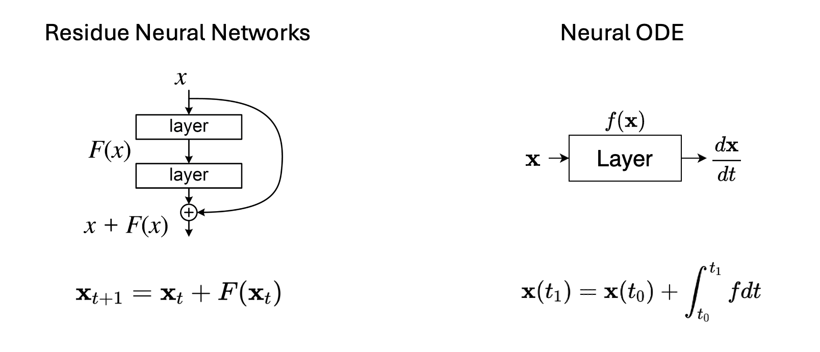
Neural Ordinary Differential Equations (ODEs) represent a subset of deep neural network models where the derivative of the hidden state is defined by a neural network, departing from the traditional approach of stacking hidden layers. In essence, neural networks parameterize the underlying differential equations, and the network’s output is computed using specialized solvers for these equations. Consequently, the primary challenge in training lies in effectively computing gradients of the target function with respect to the network parameters. And with different types of loss functions, there can be tiny modifications in the adjoint dynamic systems.
Problem Setup
Say we have a neural network parameterizing the gradients as:
\[f_{\theta}(\mathbf{z}) = \frac{d\mathbf{z}}{dt} \tag{1}\]\(f_{\theta}\) is the neural network with trainable parameters \(\theta\). The output of the model can be obtained from a black-box ODEsolver:
\[\mathbf{z}\left(t_1\right)=\text { ODESolve }\left(\mathbf{z}\left(t_0\right), f, t_0, t_1, \theta\right) \tag{2}\]Throughout history, various ODE solvers have been developed, with Euler's method and the Runge-Kutta Method standing as the two primary approaches. Selecting different ODE solvers can offer a balanced compromise between computational performance and solution accuracy.
Let’s say our target function is only a function of model output, which is the case in many supervised learning setups:
\[L\left(\mathbf{z}\left(t_1\right)\right)=L\left(\int_{t_0}^{t_1} f(\mathbf{z}(t), t, \theta) d t\right)=L\left(\operatorname{ODESolve}\left(\mathbf{z}\left(t_0\right), f, t_0, t_1, \theta\right)\right) \tag{3}\]If we want \(\underset{\theta}{\operatorname{argmin}} L\left(z\left(t_1\right)\right)\) using a gradient descent optimizer, that means we need to compute the following in an efficient way:
\[\frac{d L}{d \theta} \tag{4}\]Applying chain rule to equation (4) we have:
\[\frac{\mathrm{d} L}{\mathrm{~d} \theta}=\frac{\partial L}{\partial z\left(t_1\right)}\frac{\mathrm{d} z\left(t_1\right)}{\mathrm{d} \theta}\]But naively \(\frac{\mathrm{d} z\left(t_1\right)}{\mathrm{d} \theta}\) would require to store every intermediate states of the ODEsolver, which can be expensive and not practical at all.
There can be other more complex cases of target functions, like: $$ L(\mathbf{z}, \theta)=\int_{t_0}^{t_1} l(\mathbf{z}, \theta, t) d t $$ which appears in the maximum likelihood training of the continuous normalizing flow. And even more generally: $$ L(\mathbf{z}, \theta, t) $$ which could be picutured as the target regarding observables from MD trajectory. We will cover their training protocols in the following sections.
Adjoint Method from Lagrangian Multiplier
Reforumalte our optimization problem into a constrained optimization setup:
\[\underset{\theta}{\operatorname{argmin}} L\left({z}\left(t_1\right)\right) \\ \begin{gathered} s.t. \quad F(\dot{z (t)}, z(t), \theta, t)=\dot{z}(t)-f(z(t), \theta, t)=0 \\ z\left(t_0\right)=z_{t_0} \quad t_0<t_1 \end{gathered}\]Where the two constraints are IVP ODE system. So we can define the following function with lagrangian multiplier:
\[\psi=L\left(z\left(t_1\right)\right)-\int_{t_0}^{t_1} a(t) F(z(t), z(t), \theta, t) d t \tag{5}\]satisfying:
\[\frac{\mathrm{d} \psi}{\mathrm{d} \theta}=\frac{\mathrm{d} L\left(z\left(t_1\right)\right)}{\mathrm{d} \theta} \tag{6}\]So our target in equation (4) has changed to target in equation (6).
Do the following derivations of the second term of \(\psi\), using part integral:
\[\int_{t_0}^{t_1} a(t) F d t =a\left(t_1\right) z\left(t_1\right)-a\left(t_0\right) z_{t_0} -\int_{t_0}^{t_1}(z \dot{a}+a f) d t\]Consequently we have:
\[\begin{aligned} \frac{\mathrm{d}}{\mathrm{d} \theta}\left[\int_{t_0}^{t_1} a F d t\right]= & a\left(t_1\right) \textcolor{#fc8d62}{\frac{\mathrm{d} z\left(t_1\right)}{\mathrm{d} \theta}}-\int_{t_0}^{t_1}\left(\dot{a}+a \frac{\partial f}{\partial }\right) \textcolor{#8da0cb}{\frac{\mathrm{d} z(t)}{\mathrm{~d} \theta}} d t -\int_{t_0}^{t_1} a \frac{\partial f}{\partial \theta} d t \end{aligned}\]taking back to equation (5) we have:
\[\frac{\mathrm{d} \psi}{\mathrm{d} \theta}=\left[\frac{\partial L}{\partial z\left(t_1\right)}-a\left(t_1\right)\right] \textcolor{#fc8d62}{\frac{\mathrm{d} z\left(t_1\right)}{\mathrm{d} \theta}}+\int_{t_0}^{t_1}\left(\dot{a}(t)+a(t) \frac{\partial f}{\partial z}\right) \textcolor{#8da0cb}{\frac{\mathrm{d} z(t)}{\mathrm{d} \theta}} d t+\int_{t_0}^{t_1} a(t) \frac{\partial f}{\partial \theta} d t\]As we mentioned above, \(\textcolor{#fc8d62}{\frac{\mathrm{d} z\left(t_1\right)}{\mathrm{d} \theta}}\) and \(\textcolor{#8da0cb}{\frac{\mathrm{d} z(t)}{\mathrm{d} \theta}}\) are expensive to compute. But here we have the freedom to choose appropriate function \(a(t)\) to cancel the coefficients before both terms. That is to say:
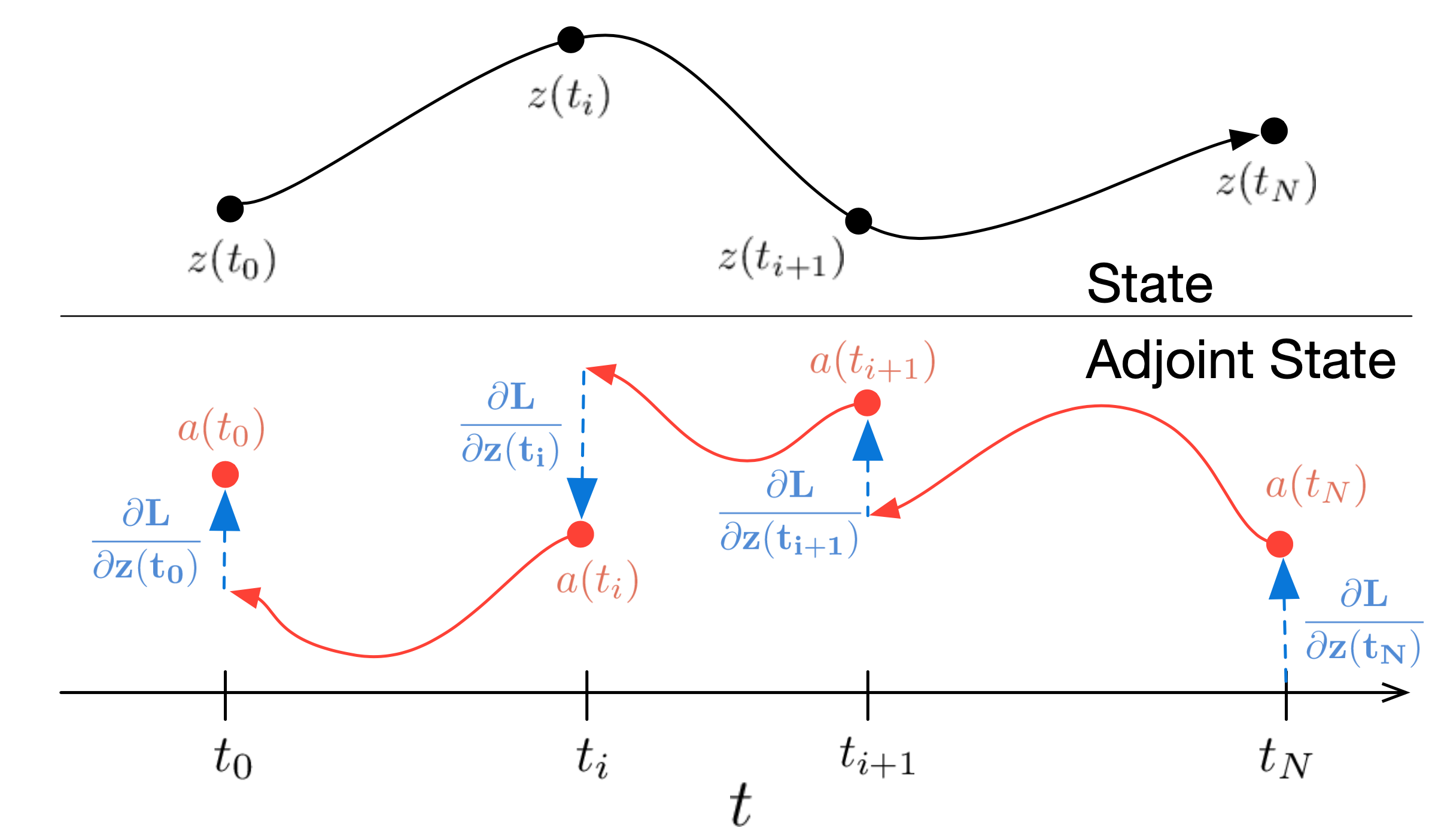
\[\left\{\begin{array}{l} \dot{a}(t)=-a(t)^{\top} \frac{\partial f}{\partial \mathbf{z}} \\[2ex] a\left(t_1\right)=\frac{\partial L}{\partial z\left(t_1\right)} \end{array}\right. \tag{7}\]which defined an adjoint dynamic system \(a\) in the reverse direction:
\[a\left(t_0\right)=a\left(t_1\right)-\int_{t_1}^{t_0} a(t) \frac{\partial f}{\partial z} d t \tag{8}\]And once we have the function \(a(t)\) from the above system, the gradient can be calculated with:
\[\frac{\mathrm{d} L}{\mathrm{~d} \theta}=\frac{\mathrm{d} \psi}{\mathrm{~d} \theta} = -\int_{t_1}^{t_0} a(t) \frac{\partial f}{\partial \theta} dt \tag{9}\]Training Algorithm

Summarize the above adjoint method into a training algorithm. Basically for target function only based on the final output \(L\left(\mathbf{z}\left(t_1\right)\right)\), a single training step involves one forward pass and two reverse passes of the ODESolver:
-
Forward pass: Solve the ODE from the time \(t_0\) to \(t_1\), get the output \(z(t_1)\)
\[\frac{d \mathbf{z}(t)}{d t}=f(\mathbf{z}(t), t, \theta), \quad \mathbf{z}\left(t_1\right)=\mathbf{z}\left(t_0\right)+\int_{t_0}^{t_1} f d t\] -
Calculate loss function \(L\left(\mathbf{z}\left(t_1\right)\right)\).
-
Backward pass: Solve ODEs from time \(t_1\) to \(t_0\) to get the gradient of the loss:
\(a(t)=-a(t) \frac{\partial f}{\partial z} \text { s.t. } a\left(t_1\right)=\frac{\partial L}{\partial z\left(t_1\right)}\) giving \(a\left(t_0\right)=a\left(t_1\right)-\int_{t_1}^{t_0} a(t) \frac{\partial f}{\partial z} d t\)
and
\[\frac{\mathrm{d} L}{\mathrm{~d} \theta}=-\int_{t_1}^{t_0} a(t) \frac{\partial f}{\partial \theta} d t\] -
Use the gradient to update the network parameters \(\theta\).
As you can see, even though the adjoint method has made the training possible, but it is still quite expensive and non-scalable because of the multiple ODESolver runs per iteration. That is where flow-matching method comes in. We will cover in the next blog.
Adjoint system for other two kinds of loss
As I mentioned above, there can be other more complex cases of target functions, which could involve more than the final output.
For example, in the maximum likelihood of continuous normalizing flow training, the target function could be written as:
\[-\underset{z_1 \sim \rho\left(z_1\right)}{\mathbb{E}}\left[\log \mu_{z_0}\left(F_{1 \rightarrow 0}\left(z_1\right)\right)+\int_0^1 \operatorname{tr}\left(\frac{\partial f}{\partial z}\right) d t\right]\]The second term in the target function involves an integration of a function of \(z\) over time, generally in this form:
\[L(\mathbf{z}, \theta)=\int_{t_0}^{t_1} l(\mathbf{z}, \theta, t) d t\]Under this circumstance, the adjoint system will be:
\[\left\{\begin{array}{l} -\dot{a}(t)-a(t)^{\top} \frac{\partial f}{\partial \mathbf{z}}+\frac{\partial l}{\partial \mathbf{z}}=0 \\ a\left(t_1\right)=0 \end{array}\right.\]and the gradient expression is:
\[\frac{d L}{d \theta}=\frac{\partial L}{\partial \theta}-\int_{t_0}^{t_1} a(t)^{\top} \frac{\partial h}{\partial \theta} d t\]The other more general form of target function is:
\[L(\mathbf{z}, \theta, t)\]And the corresponding adjoint dynamic system is:
\[\left\{\begin{array}{l} \dot{a}(t)=-a(t)^{\top} \frac{\partial f}{\partial \mathbf{z}} \\ a\left(t_i\right)=a_{t_i} \end{array}\right.\]with the gradient expression as:
\[\frac{d L}{d \theta}=\frac{\partial L}{\partial \theta}-\int_{t_0}^{t_1} a(t)^{\top} \frac{\partial h}{\partial \theta} d t\]The training algorithm is similar to above, but with different adjoint system and gradient expression.
References