Implicit Reparameterization Gradients

Deriving gradients from stochastics operations is a persistent headache in various tasks related to Bayesian inference or training generative models. The reparameterization trick has come to our rescue in numerous cases involving continuous random variables, such as the Gaussian distribution. However, many distributions lacking a location-scale parameterization or a tractable inverse cumulative function—like truncated, mixture, Von Mises or Dirichlet distributions—can’t be used with reparameterization gradients. The authors proposed an alternative approach called implicit reparameterization trick, in contrast to the classic reparameterization trick, which provided unbiased estimators for continuous distributions with numerically tractable CDFs.

Update @ Nov 23, 2023 : Attach pytorch codes to demo implicit reparameterization with customized gradient

Reference

Figurnov, Mikhail, Shakir Mohamed, and Andriy Mnih. “Implicit reparameterization gradients.” Advances in neural information processing systems 31 (2018)

Explicit Reparameterization Gradients

First let’s do a problem setup for the explicit reparameterization trick. Suppose we would like to optimize the following expectation w.r.t the distribution parameter \(\phi\):

\(f(z)\) is a continuously differentiable function.

Why this is important?
Equation (1) is quite common in stochastic variational inference for latent variable models. Except for a few special cases (like normalizing flow), the maximum likelihood target is intractable. Instead variational inference provides an alternative by introducing a surrogate posterior distribution $$q_\phi(\boldsymbol{z} \mid \boldsymbol{x})$$ and maximizing the following Evidence Lower Bound Objective (ELBO): $$ \mathcal{L}(\boldsymbol{x}, \boldsymbol{\theta}, \boldsymbol{\phi})=\mathbb{E}_{q_{\boldsymbol{\phi}}(\boldsymbol{z} \mid \boldsymbol{x})}\left[\log p_{\boldsymbol{\theta}}(\boldsymbol{x} \mid \boldsymbol{z})\right]-\mathrm{KL}\left(q_{\boldsymbol{\phi}}(\boldsymbol{z} \mid \boldsymbol{x}) \| p(\boldsymbol{z})\right) \leq \log p_{\boldsymbol{\theta}}(\boldsymbol{x}) $$ The first term is exactly in the form of equation (1) and its gradients are typically intractable and approximated using samples from the variational posterior. The reparameterization trick usually provides a low variance gradient estimator.

Assume we can find a standardize function \(\mathcal{S}_\phi(\boldsymbol{z})\) differentiable to \(\phi\) and also invertible:

It will remove \(z\)’s dependence on the parameters of the distribution. Then we can do:

The dependence on \(\phi\) has been moved into \(f\), so the gradient is tractable:

Why CDF is an universal standardization function?
For an arbitrary univariant distribution \(q_\phi(\boldsymbol{z})\), the cumulative distribution function (CDF) \(F(z|\phi)\) convert the distribution to a parameter-indpendent uniform distribution: $$ \mathcal{S}_\phi(z)=F(z \mid \phi) \sim \text { Uniform }(0,1) $$ By the way, if the inverse CDF is attractable, that also means you can easily do one-shot batch sampling of the target distribution: first do one-shot sampling with uniform distribution and apply inverse CDF. For multivariate case, the distribution transform looks like: $$ \mathcal{S}_{\boldsymbol{\phi}}(\boldsymbol{z})=\left(F\left(z_1 \mid \boldsymbol{\phi}\right), F\left(z_2 \mid z_1, \boldsymbol{\phi}\right), \ldots, F\left(z_D \mid z_1, \ldots, z_{D-1}, \boldsymbol{\phi}\right)\right)=\boldsymbol{\varepsilon} $$ where \(q(\varepsilon)=\prod_{d=1}^D \text { Uniform }\left(\varepsilon_d \mid 0,1\right)\).

However, it is not always practical to find an invertible and tractable standardization function. For example, Rice distribution \(f(x \mid \nu, \sigma)=\frac{x}{\sigma^2} \exp \left(\frac{-\left(x^2+\nu^2\right)}{2 \sigma^2}\right) I_0\left(\frac{x \nu}{\sigma^2}\right)\) is important in scattering and wireless communication field. The CDF is \(1-Q_1\left(\frac{\nu}{\sigma}, \frac{x}{\sigma}\right)\), where \(Q_1\) is the Marcum Q-function. So currently the inverse CDF is not tractable.

Implicit Reparameterization Gradients

The authors porposed an alternative way for the raparameterization gradient that avoids the inversion of the standardization function. Start from Equation (4):

Key point is compute \(\nabla_\phi z\) by implicit differentiation. Apply total gradient \(\nabla_{\boldsymbol{\phi}}^{\mathrm{TD}}\) to the equality \(\mathcal{S}_\phi(\boldsymbol{z})=\boldsymbol{\varepsilon}\), you got:

Now the gradient only requires differentiating the standardization function and not inverting it. Say if we use the CDF as an universal standardization function for an arbitrary distribution \(q_{\phi}(z)\), we have:

Algorithm
$$ \begin{array}{lll} \hline & \text { Explicit reparameterization } & \text { Implicit reparameterization } \\ \hline \text { Forward pass } & \begin{aligned} &\text { Sample } \boldsymbol{\varepsilon} \sim q(\boldsymbol{\varepsilon}) \\ &\text { Set } \boldsymbol{z} \leftarrow \mathcal{S}_{\boldsymbol{\phi}}^{-1}(\boldsymbol{\varepsilon}) \end{aligned} & \text { Sample } \boldsymbol{z} \sim q_{\boldsymbol{\phi}}(\boldsymbol{z}) \\ \hline \text { Backward pass } & \begin{aligned} &\text { Set } \nabla_{\boldsymbol{\phi}} \boldsymbol{z} \leftarrow \nabla_\phi \mathcal{S}_{\boldsymbol{\phi}}^{-1}(\boldsymbol{\varepsilon}) \\ &\text { Set } \nabla_{\boldsymbol{\phi}} f(\boldsymbol{z}) \leftarrow \nabla_{\boldsymbol{z}} f(\boldsymbol{z}) \nabla_{\boldsymbol{\phi}} \boldsymbol{z} \end{aligned} & \begin{aligned} &\text { Set } \nabla_{\boldsymbol{\phi}} \boldsymbol{z} \leftarrow-\left(\nabla_{\boldsymbol{z}} \mathcal{S}_{\boldsymbol{\phi}}(\boldsymbol{z})\right)^{-1} \nabla_\phi \mathcal{S}_{\boldsymbol{\phi}}(\boldsymbol{z}) \\ &\text { Set } \nabla_{\boldsymbol{\phi}} f(\boldsymbol{z}) \leftarrow \nabla_{\boldsymbol{z}} f(\boldsymbol{z}) \nabla_{\boldsymbol{\phi}} \boldsymbol{z} \end{aligned} \\ \hline \end{array} $$

Pytorch Implementation Example

The following demonstrates the implementation of implicit reparameterization using a Gaussian distribution. It serves as a framework example, considering that Gaussian distribution already possesses a clearly established explicit reparameterization technique. To apply implicit reparameterization sampling to other distributions, you require three key components: a differentiable cumulative distribution function (CDF), various methods for sampling from the distribution, and a probability density function (PDF).

class NormalIRSample(torch.autograd.Function):
    @staticmethod
    def forward(ctx, loc, scale, samples, dFdmu, dFdsig, q):
        dzdmu = -dFdmu/q
        dzdsig = -dFdsig/q
        ctx.save_for_backward(dzdmu, dzdsig)
        return samples

    @staticmethod
    def backward(ctx, grad_output):
        dzdmu, dzdsig, = ctx.saved_tensors
        return grad_output * dzdmu, grad_output * dzdsig, None, None, None, None

class IRNormal(torch.distributions.Normal):
    def __init__(self, *args, **kwargs):
        super(IRNormal, self).__init__(*args, **kwargs)
        self._irsample = NormalIRSample().apply

    def pdf(self, value):
        return torch.exp(self.log_prob(value))

    def irsample(self, sample_shape=torch.Size()):
        samples = self.sample(sample_shape) # sample without grad
        F = self.cdf(samples)
        q = self.pdf(samples)
        dFdmu = torch.autograd.grad(F, self.loc, retain_graph=True)[0]
        dFdsig = torch.autograd.grad(F, self.scale, retain_graph=True)[0]
        samples.requires_grad_(True)
        return self._irsample(self.loc, self.scale, samples, dFdmu, dFdsig, q)

And it works as:

>>> mu = torch.tensor(1.0, requires_grad=True)
>>> sig = torch.tensor(2.0, requires_grad=True)
>>> dista = IRNormal(mu, sig)
>>> z = dista.irsample()
>>> z
tensor(1.9856, grad_fn=<NormalIRSampleBackward>)
>>> z.backward()
>>> mu.grad
tensor(1.0000)
>>> sig.grad
tensor(0.4928)

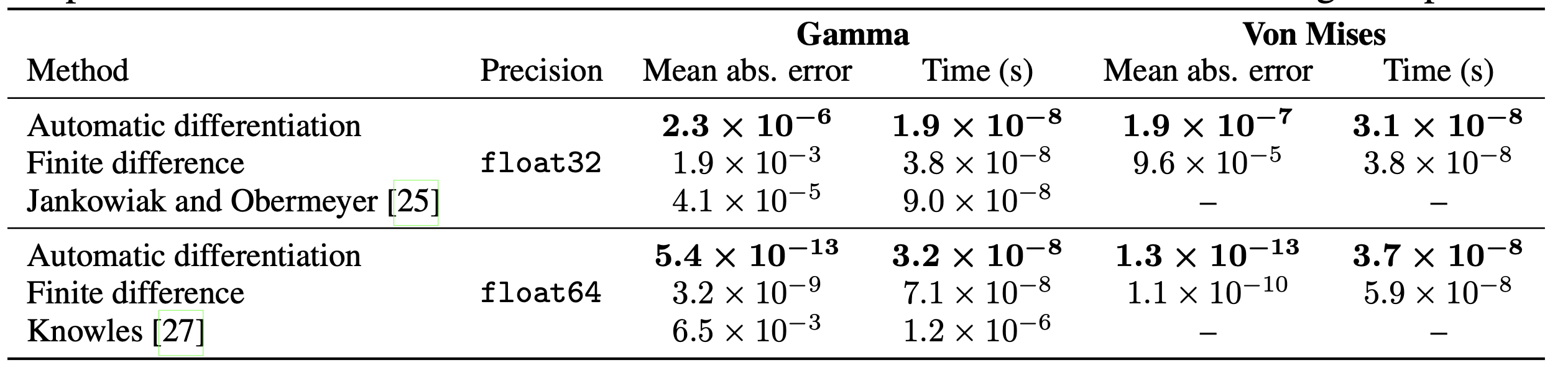
Accuracy and speed of reparameterization gradient estimators

In this paper, the author compared the implicit reparameterization estimator with two alternatives, Automatic differentiation with implicit reparameterization achieves the lowest error and the highest speed.