Early Implementation of Attention Mechanism

[  AI&Physics  Attention  ] 27 Dec 2021

We are witnessing the popularity and fast development of the Attention Mechanism in the deep learning community in recent years. It serves as the pivotal parts in most state-of-the-art models in NLP tasks, and continues to be a rapid evolving research topics in CV field. Besides, in recent AI-related scientific breakthroughs, like AlphaFold 2, the Attention Mechanism looks like an omnipresent component in the models. That is why we (Kevin and I) decided to start a journal club to read and discuss seminal papers about how attention was introduced and further developed. We hope this discussion could bring us more intuition about this fancy name, such that we could apply it to problems we are interested in with more confidence.

This blog is a note of the first discussion, about the paper Bahdanau, et al. (2014) Neural machine translation by jointly learning to align and translate¹. As an early (or first) implementation of “Attention Mechanism” in the translation task, it helps a lot, at least for me, to understand what is attention, although the attention here is a little different from that in the following Transformer model.

1. Translation Task and Previous Seq2Seq Model
   1. RNN Encoder
   2. RNN Decoder
   3. Beam Search
   4. Problem of the Seq2Seq Model
2. Introduce Attention to the model
   1. Modify the context vector \(c\) in Decoder
   2. Bi-Directional RNN as the Encoder
   3. Results
3. Discussion
4. References

Translation Task and Previous Seq2Seq Model

People are trying to translate natural languages with machines. There are two major approaches in machine translation tasks: Traditional phrase-based translation system consists of many small sub-components that are tuned separately; Neural machine translation aims at building a single neural network that can be jointly tuned to maximize the translation performance.

Before the publication of this attention mechanism paper, Seq2Seq model² achieved the best results in neural translation tasks. And in fact, the attention mechanism is only a tiny but profound modification to the Seq2Seq model. So we will first review the Seq2Seq Model’s architecture and limitations, then the introduction of the “attention” would be intuitive.

Seq2Seq Model belongs to a family of encoder-decoders in the neural machine translation approach. They typically encode a source sentence into a fixed-length vector, from which a decoder generates a translation.

RNN Encoder

Say we have the source sentence \(\mathbf{x}\) and the output sentence \(\mathbf{y}\):

\[\mathbf{x}=\left(x_{1}, \ldots, x_{T_{x}}\right), x_{i} \in \mathbb{R}^{K_{x}} \\ \mathbf{y}=\left(y_{1}, \ldots, y_{T_{y}}\right), y_{i} \in \mathbb{R}^{K_{y}} \tag{1}\]

Each natural language sentence will first be tokenized (usually includes an ending signal), and each word or token into fixed length vectors. But apparently, different sentences could have different lengths \(T_x\) and \(T_y\)

The encoder reads input sequence \(\mathbf{x}=\left(x_{1}, \ldots, x_{T_{x}}\right), x_{i}\), and pass through a RNN (Recurrent Neural Network) like:

\[h_{t}= \begin{cases}f\left(x_{t}, h_{t-1}\right) & , \text { if } t>0 \\ 0 & , \text { if } t=0\end{cases} \tag{2}\]

where \(h_t \in \mathbb{R}^n\) is a hidden state at time \(t\) and \(f\) are non linear functions. This iterative path will output a series of hidden states:

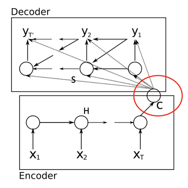
\[H=\left(h_{1}, \cdots, h_{T_{x}}\right), h_{i} \in \mathbb{R}^{n}\]

Generally, a context vector \(c\) will be generated from the hidden states with another nonlinear function \(q\), as shown in figure 1³:

\[c= q(\{h_1,\dots,h_{T_x}\}) = h_T\tag{3}\]

Usually they use the LSTM as the \(f\).

It is intuitive to choose \(c=h_T\) at the moment, as \(h_T\) is the only hidden state which could possibly contain all information in the source sentence. But this is not a perfect choice of course, as we all know now RNN would concentrate more on the information around the node.

RNN Decoder

The decoder is often trained to predict the next word \(y_{i}\) given the context vector \(c\) and previously predicted words \(\{y_1, \dots, y_{i-1}\}\).

Again, as this is a RNN, hidden states also exist in the decoder part, generated from the previous hidden state, previous predicted word and the context vector:

\[s_{i}=f\left(s_{i-1}, y_{i-1}, c\right) \tag{4}\]

Then the conditional probability predict of the next word will be:

\[p\left(y_{i} \mid y_{1}, \ldots, y_{i-1}, \mathbf{x}\right)=g\left(y_i \mid y_{i-1}, s_{i}, c\right) \tag{5}\]

During the training process, loss function is constructed to maximize the likelihood of the true next word. Once the model is trained, they usually use algorithms like beam search that approximately maximizes the conditional probability to predict the output sentences.

Beam Search

This is not related to attention, but I found it an interesting and common algorithm in machine translation tasks. Once the model is trained, at each time step of the decoder, they keep the \(s\) candidates with the highest log-probability, where \(s\) is the beam-width. During the beam-search, they exclude any hypothesis that includes an unknown word. For each end-of-sequence symbol that is selected among the highest scoring candidates the beam-width is reduced by one, until the beam-width reaches zero.⁴

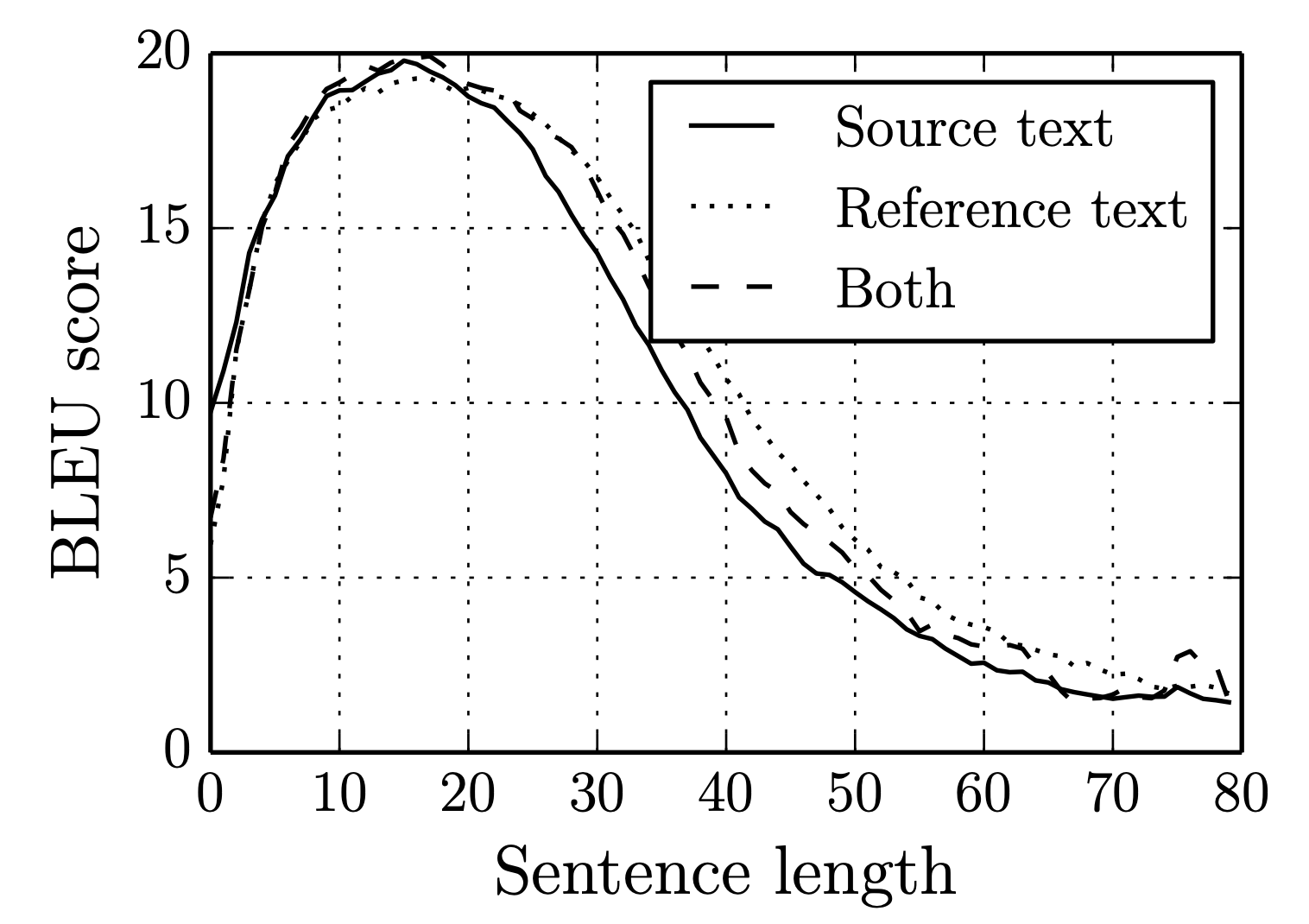
Problem of the Seq2Seq Model

As indicated by the equation (4) and (5), a single context vector \(c\) is used in prediction for all \(s_i\) and \(y_i\). That means, the RNN encoder needs to compress all the necessary information of the source sentence into a single fixed-length vector. It is not surprising that the Seq2Seq model can hardly cope with long sentences, as shown in figure 2⁴. Fixing this issue is the motivation of the paper.

Introduce Attention to the model

Modify the context vector \(c\) in Decoder

As the bottleneck for the previous Seq2Seq Model is the single context vector \(c\) for all \(y_i\) and \(s_i\) prediction, it is intuitive to modify the above equation (3) into:

\[c_{i}=\sum_{j=1}^{T_{x}} \alpha_{i j} h_{j} \tag{6}\]

This is just a weighted sum of the hidden states.

The weights \(\alpha_{ij}\) is constructed as following: $$ \alpha_{i j}=\frac{\exp \left(e_{i j}\right)}{\sum_{k=1}^{T_{x}} \exp \left(e_{i k}\right)} \\[2ex] e_{i j}=v_{a}^{\top} \tanh \left(W_{a} s_{i-1}+U_{a} h_{j}\right) $$ where \(v_{a} \in \mathbb{R}^{n^{\prime}}, W_{a} \in \mathbb{R}^{n^{\prime} \times n}\) and \(U_{a} \in \mathbb{R}^{n^{\prime} \times 2 n}\) are trainable weight matrices. Here the \(s_{i-1}\) and \(h_j\), as defined previously, are (i-1)-th and j-th elements in the hidden states of input and output.
So the weights \(\alpha_{ij}\) can be understood as an alignment between the input j and output i. That's why the title of the paper is "jointly learning to align and translate".

And accordingly change the equation (4) and (5) into:

\[\begin{aligned} s_{i}&=f\left(s_{i-1}, y_{i-1}, c_{i}\right) \\ p\left(y_{i} \mid y_{1}, \ldots, y_{i-1}, \mathbf{x}\right)&=g\left(y_{i-1}, s_{i}, c_{i}\right) \end{aligned} \tag{7}\]

The above modification means, now for each output \(y_i\), we have a separate context vector \(c_i\), which comes from a weighted sum of all hidden states.

In this paper, they call this weighted sum (6) as “attention”, which is not surprising as different output \(y_i\) would probably focus on different parts of the inputs controlled by the trainable weights:

The probability \(\alpha_{i j}\), or its associated energy \(e_{i j}\), reflects the importance of the annotation \(h_{j}\) with respect to the previous hidden state \(s_{i-1}\) in deciding the next state \(s_{i}\) and generating \(y_{i}\). Intuitively, this implements a mechanism of attention in the decoder. The decoder decides parts of the source sentence to pay attention to. By letting the decoder have an attention mechanism, we relieve the encoder from the burden of having to encode all information in the source sentence into a fixed-length vector. With this new approach the information can be spread throughout the sequence of annotations, which can be selectively retrieved by the decoder accordingly.

Bi-Directional RNN as the Encoder

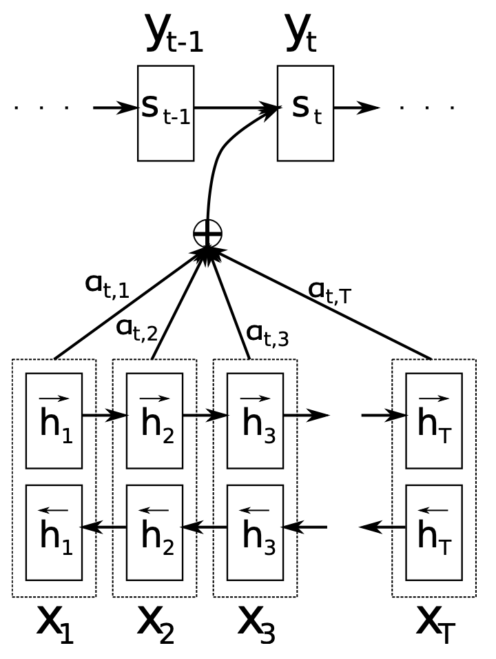
Another trick serves as a complement to the above attention mechanism: Bi-Directional RNN. Think about the motivation of equation (6), we hope that the \(\alpha_{ij}\) could be more like a correlation between input \(j\) and output \(i\). But in the previous RNN Encoder, as shown in equation (2) and Figure 1, different hidden states \(h_j\) does not contain same amount of information. For example, \(h_j\) only contains information from input \(x_1\) to \(x_{j-1}\). They are not fair bases to define a weighted sum, as of course the last \(h_{Tx}\) contains the most knowledge. The desideratum here is that, each \(h_j\) has similar amount of information, and with a focus on the input \(x_j\).

Bi-Directional RNN is a natural way to make this happen. The math now works as the following with a forward and backward RNN:

\[\vec{h}_{t}= \begin{cases}f\left(x_{t}, \vec{h}_{t-1}\right) & , \text { if } t>0 \\ 0 & , \text { if } t=0\end{cases} \quad \quad \overleftarrow{h}_{t}= \begin{cases}f\left(x_{t}, \overleftarrow{h}_{t+1}\right) & , \text { if } t<T_{x} \\ 0 & , \text { if } t=T_{x}\end{cases} \tag{8}\]

And they concatenate the above two to construct the hidden state:

\[h_{j}=\left[\vec{h}_{j}^{\top} ; \overleftarrow{h}_{j}^{\top}\right] \tag{9}\]

Now, theoretically, \(h_j\) should include information about from \(x_1\) to \(x_{Tx}\) with a focus on the \(x_j\), which is what we want. The overall modified Seq2Seq model is shown in Figure 3¹:

Results

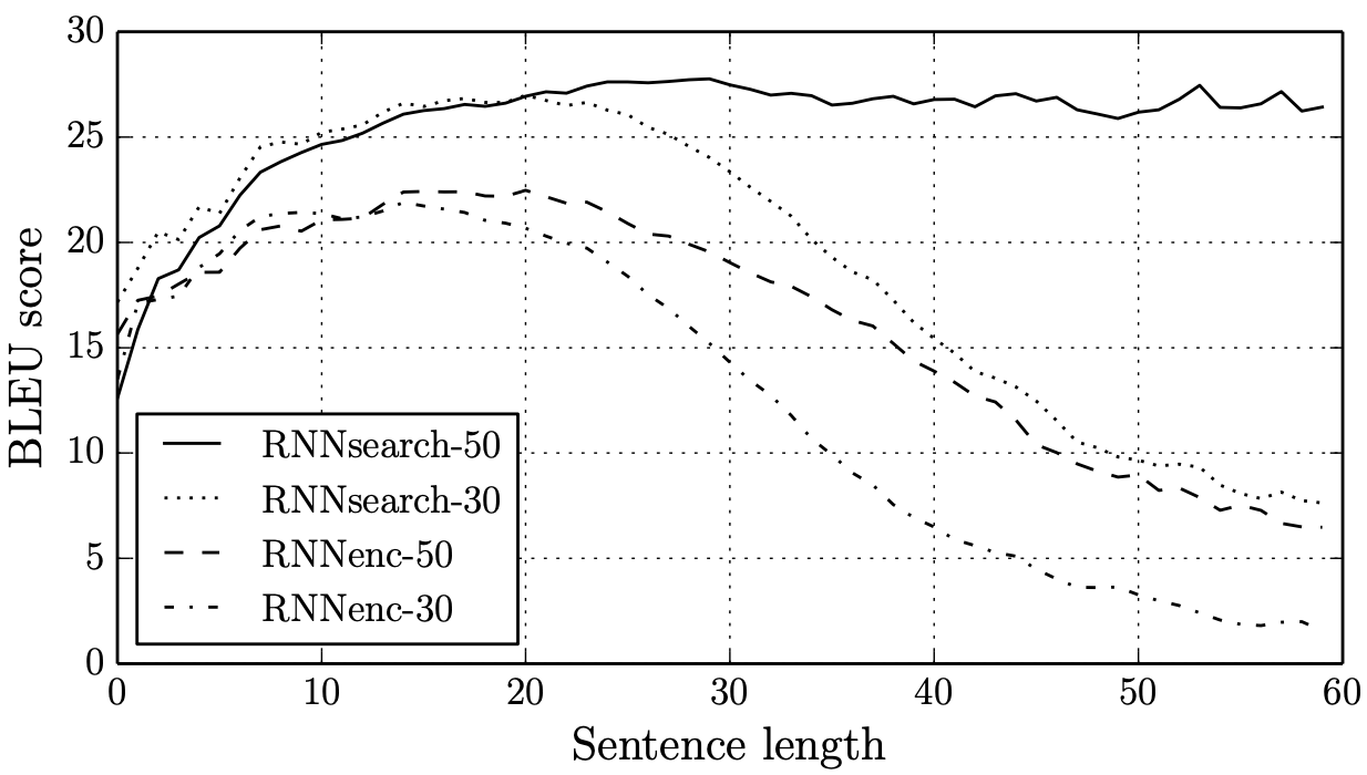
With the above two modifications, the new model works much better on longer sentences, as shown in Figure 4¹

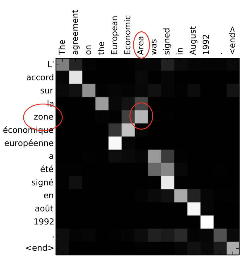
Besides the visualizaion of weights \(\alpha_{ij}\) in the attention equation (6) makes the model more interpretable, as the alignment between the input and output appears exactly as it should be in Figure 5¹:

Discussion

Given the above discussion, let’s come back to the question: What is attention? Why it is powerful? Clearly for me, from the equation (6), attention is more like explicily writing out and optimize the correlation weights you are interested in. Here we want the correlation (alignment) between the input and output words, so the format like equation (6) did the job. Theoretically, DNN itself could capture the correlation with its abundant weights, but explicitly writing out and optimizing the specific correlations you are interested in seems important. From my point of view, the reason why attention is useful is similar to that why CNN works better on CV tasks than naive MLPs.

In this paper, we write out the correlation between the input and output, but we are still using RNN to capture the correlation between sequential elements in input. It is very natural to move one step further: what if we replace the RNN with the “attention” idea? Just explicitly write out the correlation between order elements and optimize them? Could it work better than RNN? This is the primary motivation of “self-attention” and the transformer model. We will cover this topic in a future blog.

References