Spectral Bias and Positional Encoding
26 Jul 2021Recent days (maybe it is already out of date when you read this blog), we see a “renaissance” of classic multilayer perceptron (MLP) models in machine learning field. The logic behind this trend is heuristic for researches to see that, by understanding how a complex black box works, we can naturally add some reasonably modifications to make it better, instead of shotting with blind eyes. The majority of the blog is based on paper Tancik, Matthew, et al. (2020) Fourier features let networks learn high frequency functions in low dimensional domains.
The basic take-away is, a standard MLP model fails to learn high frequencies both in theory and in practice, which is called Spectral Bias. Based on this findings, with a simple Fourier feature mapping (Positional Encoding), the performance of MLPs can be greatly improved, especially for low-dimensional regression tasks, like your inputs are atom coordinates.
- Neural Tangent Kernel
- Spectral Bias during training
- Fourier Feature and Encoding methods
- Real Applications
Neural Tangent Kernel
Kernel Regression
Kernel regression is a classic nonlinear regression algorithm. Given a training dataset \((\mathbf{X}, \mathbf{y})=\left\{\left(\mathbf{x}_{i}, y_{i}\right)\right\}_{i=1}^{n}\), where \(\mathbf{x}_{i}\) are input points and \(y_{i}=f\left(\mathbf{x}_{i}\right)\) are the corresponding scalar output labels, kernel regression constructs an estimate \(\hat{f}\) of the underlying function at any point \(\mathbf{x}\) as:
\[\hat{f}(\mathbf{x})=\sum_{i=1}^{n}\left(\mathbf{K}^{-1} \mathbf{y}\right)_{i} k\left(\mathbf{x}_{i}, \mathbf{x}\right)\tag{1}\]where \(\mathbf{K}\) is an \(n \times n\) kernel (Gram) matrix with entries \(\mathbf{K}_{i j}=k\left(\mathbf{x}_{i}, \mathbf{x}_{j}\right)\) and \(k\) is a symmetric positive semidefinite (PSD) kernel function which represents the “similarity” between two input vectors.
Intuitively, the kernel regression estimate at any point \(\mathbf{x}\) can be thought of as a weighted sum of training labels \(y_{i}\) using the similarity between the corresponding \(\mathbf{x}_{i}\) and \(\mathbf{x}\).
Approximate deep networks with kernel regression
Let \(f\) be a fully-connected nonlinear deep network with weights \(\theta\) initialized from a Gaussian distribution \(\mathcal{N}\). Theory proposed in Ref1 shows that when the width of the layers in \(f\) tends to infinity and the learning rate for SGD tends to zero, the function \(f(\mathbf{x};\theta)\) converges over the course of training to the kernel regression solution using the neural tangent kernel (NTK), defeined as:
\[k_{\mathrm{NTK}}\left(\mathbf{x}_{i}, \mathbf{x}_{j}\right)=\mathbb{E}_{\theta \sim \mathcal{N}}\left\langle\frac{\partial f\left(\mathbf{x}_{i} ; \theta\right)}{\partial \theta}, \frac{\partial f\left(\mathbf{x}_{j} ; \theta\right)}{\partial \theta}\right\rangle \tag{2}\]As the width becomes large, the neural network can be effectively replaced by its first-order Taylor expansion with respect to its parameters at initialization. For this linear model, the dynamics of gradient descent become analytically tractable.
An NTK linear system model can be used to approximate the dynamics of a deep network during training. Consider a network trained with L2 loss and a learin rate \(\eta\), where the network’s weights are initialized such taht the output of the network at initialization is close to zero. Under asymptotic conditions stated in Ref2, the output for any data \(\mathbf{X}_{\text{test}}\) after \(t\) training iterations can be approximated as:
\[\hat{\mathbf{y}}^{(t)} \approx \mathbf{K}_{\text {test }} \mathbf{K}^{-1}\left(\mathbf{I}-e^{-\eta \mathbf{K} t}\right) \mathbf{y} \tag{3}\]where \(\hat{\mathbf{y}}^{(t)}=f\left(\mathbf{X}_{\text {test }} ; \theta\right)\) are the network’s predictions on input points \(\mathbf{X}_{\text {test }}\) at training iteration \(t\), \(\mathbf{K}\) is the NTK matrix between all pairs of training points in \(\mathbf{X}\), and \(\mathbf{K}_{\text {test }}\) is the NTK matrix between all points in \(\mathbf{X}_{\text {test }}\) and all points in the training dataset \(\mathbf{X}\).
Spectral Bias during training
Let us consider the training error \(\hat{\mathbf{y}}_{\text {train }}^{(t)}-\mathbf{y}\), where \(\hat{\mathbf{y}}_{\text {train }}^{(t)}\) are the network’s predictions on the training dataset at iteration \(t\). Since the NTK matrix \(\mathbf{K}\) must be PSD, we can take its eigendecomposition \(\mathbf{K}=\mathbf{Q} \mathbf{\Lambda} \mathbf{Q}^{\mathrm{T}}\), where \(\mathbf{Q}\) is orthogonal and \(\mathbf{\Lambda}\) is a diagonal matrix whose entries are the eigenvalues \(\lambda_{i} \geq 0\) of \(\mathbf{K}\). Then, take \(e^{-\eta \mathbf{K} t}=\mathbf{Q} e^{-\eta \Lambda t} \mathbf{Q}^{\mathrm{T}}\) into equation 3:
\[\mathbf{Q}^{\mathrm{T}}\left(\hat{\mathbf{y}}_{\text {train }}^{(t)}-\mathbf{y}\right) \approx \mathbf{Q}^{\mathrm{T}}\left(\left(\mathbf{I}-e^{-\eta \mathbf{K} t}\right) \mathbf{y}-\mathbf{y}\right)=-e^{-\eta \boldsymbol{\Lambda} t} \mathbf{Q}^{\mathrm{T}} \mathbf{y} \tag{4}\]This means that if we consider training convergence in the eigenbasis of the NTK, the \(i^{\text {th }}\) component of the absolute error \(\left \vert \mathbf{Q}^{\mathrm{T}}\left(\hat{\mathbf{y}}_{\text {train }}^{(t)}-\mathbf{y}\right)\right \vert _{i}\) will decay approximately exponentially at the rate \(\eta \lambda_{i}\).
In other words, components of the target function that correspond to kernel eigenvectors with larger eigenvalues (larger wavelength, lower frequency) will be learned faster.
For a conventional MLP, the eigenvalues of the NTK decay rapidly (very low bandwidth). This results in extremely slow convergence to the high frequency components of the target function, to the point where standard MLPs are effectively unable to learn these components, as shown in the following figure (from Main Ref Figure 1).
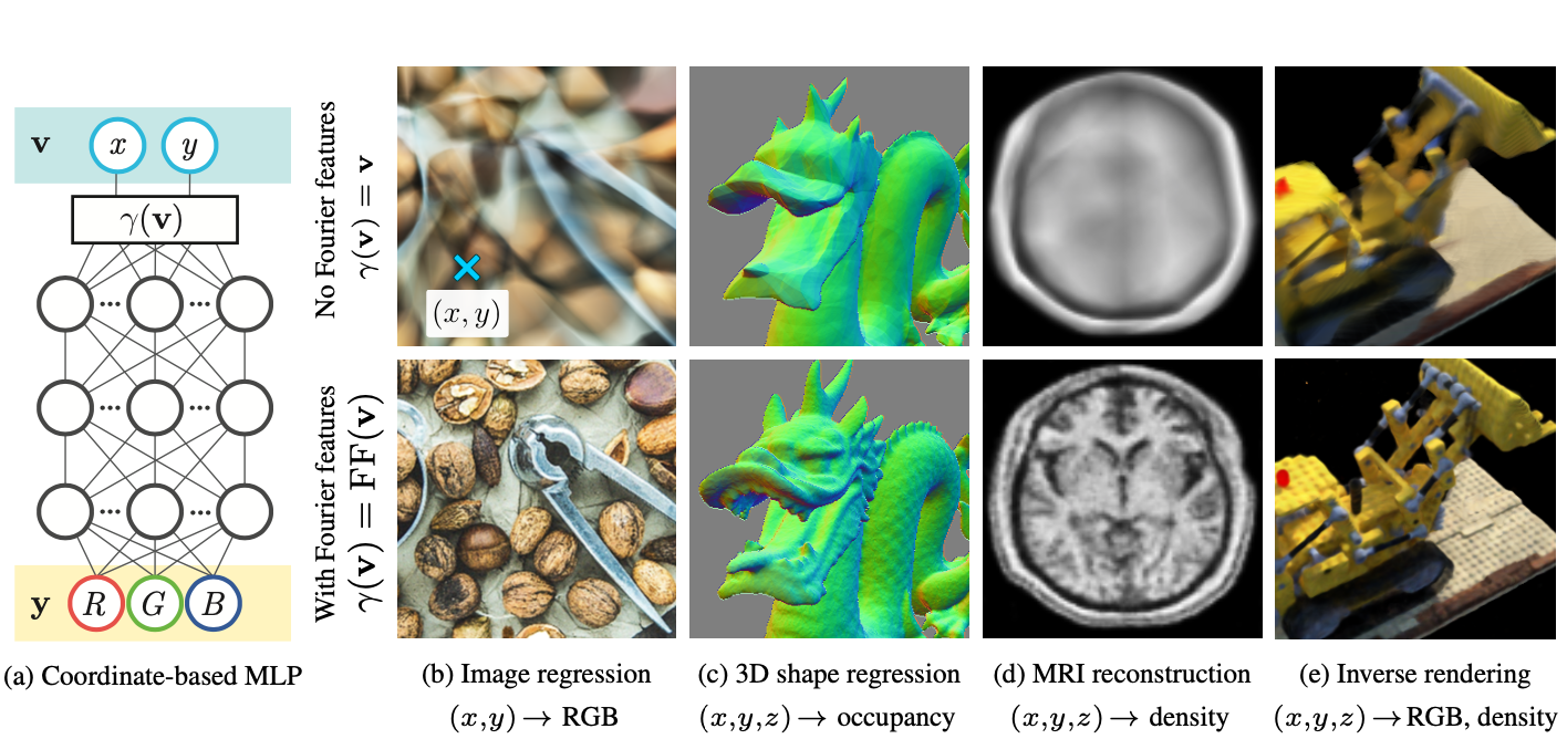
Fourier Feature and Encoding methods
The solution to the above spectral bias issue is mapping the input points into a fourier feature space with tunable bandwidth, before passing to the MLP. Say we have input points \(\mathbf{v} \in [0,1)^d\), we can map them to a higher dimensional fourier feature space with function \(\gamma\):
\[\gamma(\mathbf{v})=\left[a_{1} \cos \left(2 \pi \mathbf{b}_{1}^{\mathrm{T}} \mathbf{v}\right), a_{1} \sin \left(2 \pi \mathbf{b}_{1}^{\mathrm{T}} \mathbf{v}\right), \ldots, a_{m} \cos \left(2 \pi \mathbf{b}_{m}^{\mathrm{T}} \mathbf{v}\right), a_{m} \sin \left(2 \pi \mathbf{b}_{m}^{\mathrm{T}} \mathbf{v}\right)\right]^{\mathrm{T}} \tag{5}\]where \(\mathbf{b}_j\) are the Fourier basis frequencies, and \(a_j\) are the Fourier series coefficients. Then the MLP becomes \(f(\gamma(\mathbf{v});\theta)\).
Of course the number of terms in the Fourier feature, or the number of non-zero \(a_j\) determines the bandwidth.
Effect of Fourier Features in 1D toy system
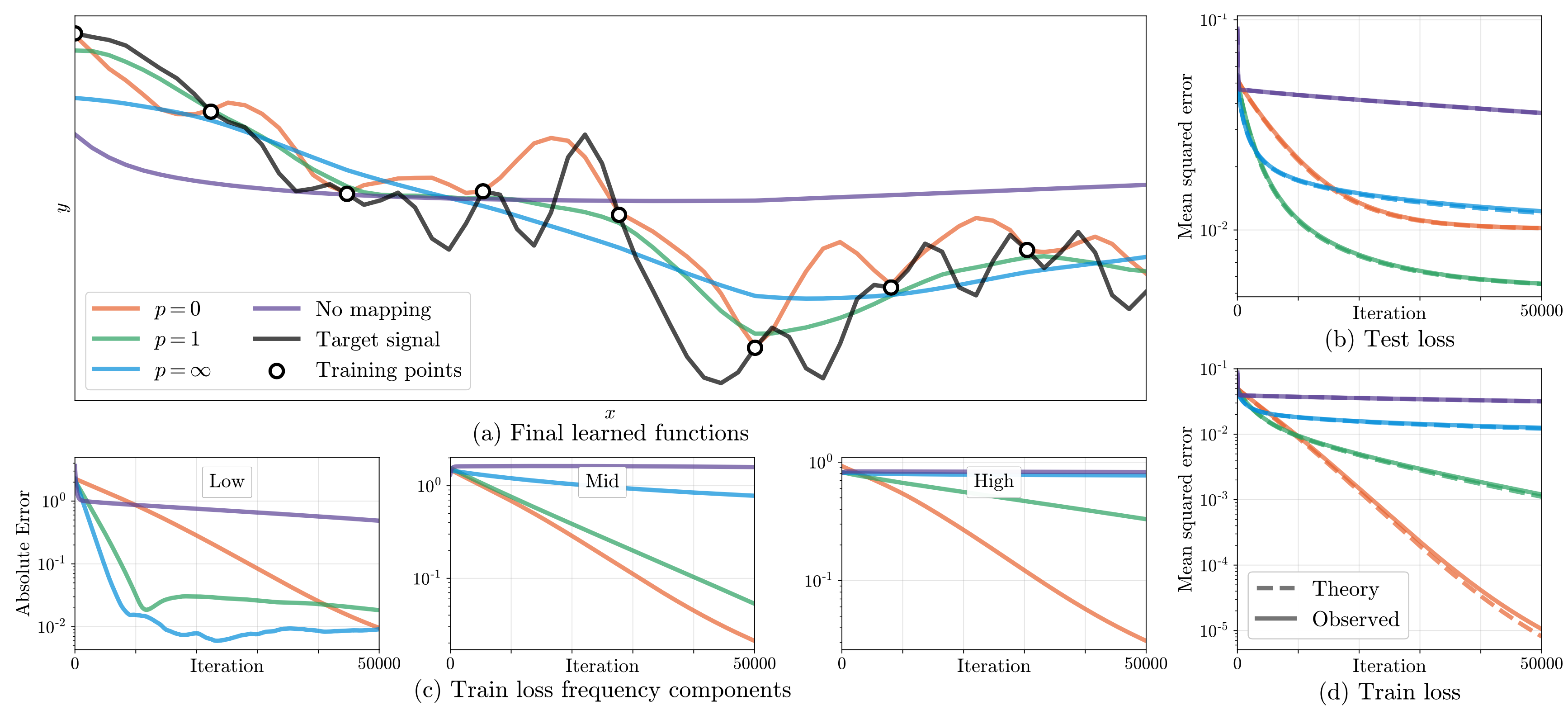
To visualize how the Fourier feature affect the model performance, we first look at a 1D toy system. Say input \(v\) is a scalar, we can then set \(b_j=j\) (as a full Fourier basis in 1D) and \(a_j = 1/j^p\) for \(j=1,\dots,n/2\) in equation 5. Apparently the adjustable parameter \(p\) determined the bandwidth of the Fourier Feature.
Smaller \(p\) means more terms in equation (5) has non-negligible coefficients (wider bandwidth), larger \(p\) means narrower bandwidth. Specially, \(p=\infty\) means the mapping \(\gamma(v) = [\cos 2\pi v, \sin 2\pi v]^T\).
The experiments in this 1D system shows that (as in the below figure, from Main Ref Figure 3): Choosing \(p\) is a tradeoff between expressiveness and overfitting, a lower \(p\) will include more high frequency features but will also give rise to overfitting. Here \(p=1\) is the optimal choice (smallest test loss).
Generalized Positional Encoding
For higher dimensional inputs, the Fourier Feature mapping can be approached by \(\gamma(\mathbf{v})=\left[\ldots, \cos \left(2 \pi \sigma^{j / m} \mathbf{v}\right), \sin \left(2 \pi \sigma^{j / m} \mathbf{v}\right), \ldots\right]^{\mathrm{T}}\), for \(j = 0, \dots, m-1\). Use log-linear spaced frequencies for each dimension. And the scale \(\sigma\) is chosen by hyperparameter sweep.
Note that this mapping is deterministic and only contains on-axis frequencies, making it naturally biased towards data that has more frequency content along the axes.
A similar mapping is used in the popular Transformer architecture, where it is also referred to as a positional encoding. However, Transformers use it for a different goal of providing the discrete positions of tokens in a sequence as input to an architecture that does not contain any notion of order. In contrast, we use these functions to map continuous input coordinates into a higher dimensional space to enable our MLP to more easily approximate a higher frequency function.
Gaussian Encoding
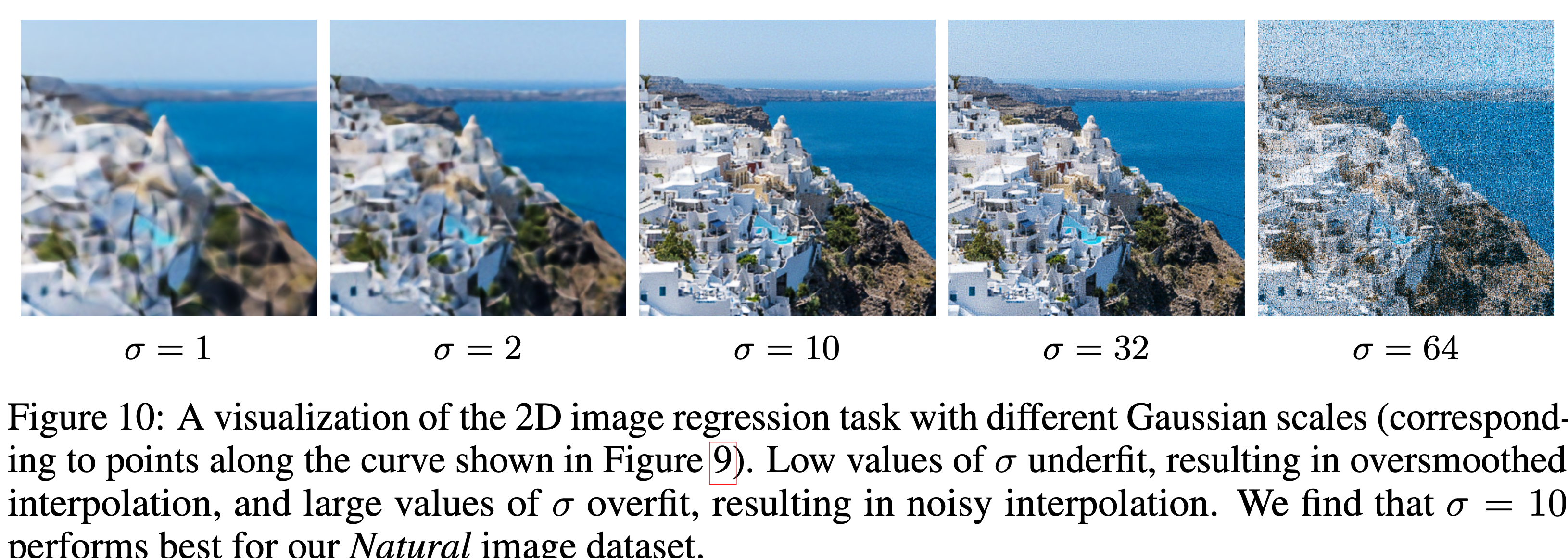
Another, and better, mapping method for higher dimensional inputs is Gaussian Encoding: \(\gamma(\mathbf{v})=[\cos (2 \pi \mathbf{B} \mathbf{v}), \sin (2 \pi \mathbf{B} \mathbf{v})]^{\mathrm{T}}\), where each entry in \(\mathbf{B}\ in \mathbb{R}^{m \times d}\) is sampled from \(\mathcal{N}(0,\sigma^2)\). The scale \(\sigma\) is chosen by hyperparameter sweep, again a tradeoff like the \(p\) above, see the figure below (From from Main Ref Figure 10).
Real Applications
Here are some real application projects showing the power of positional encodings: