Computational Theories of Sex and Recombination
15 Mar 2021This is asummary about paper Livnat, Adi, et al. (2008) A mixability theory for the role of sex in evolution. and Chastain, Erick, et al. (2014) Algorithms, games, and evolution. The two papers are targeting different central questions, but they both have a good discussion about what is the evolutionary role of sex and recombination from a computational framwork.
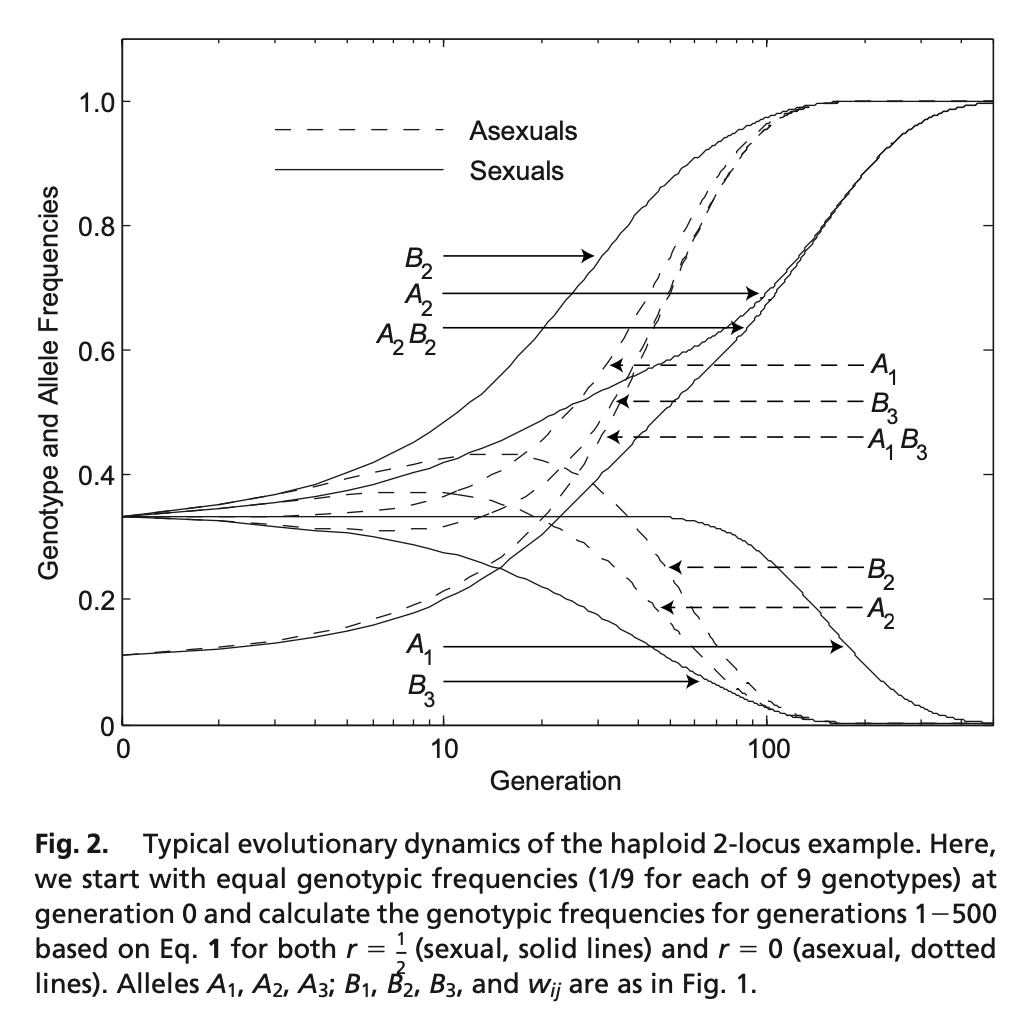
It is a long-standing question that what role sex plays in evolution. A direct answer could be, sex should help facinitate in fitness. However, even this general and abstract answer is not correct given that sometimes sex recombination break down highly favorable genetic combinations. So authors of the first paper use a computational model show that, instead of single genotypic fitness, sex recombination helps to facilitate the increase of “Mixability”, a kind of defined average fitness. Assume we have a haploid 2-locus fitness landscape as in Figure 1 below:

Let \(P_{ij,t}\) be the frequency of genotype \(A_iB_j\) at generation \(t\), \(r\) be the recombination rate (\(0\le r \le1/2\)), and \(w_{ij}\) be the fitness of \(A_iB_j\). So average fitness at generation \(t\) is:
\[\bar{w}_{t}=\sum_{i, j} P_{i j, t} w_{i j}\]and the relative fitness ratio (considering both fitness and population frequency) of genotype \(A_iB_j\) at generation \(t\) is:
\[\tilde{P}_{i j, t}=P_{i j, t} w_{i j} / \bar{w}_{t}\]They further define the following equations to describe the evolutionary dynamics of the large panmitic pupulation without mutation:
\[P_{i j, t+1}=(1-r) \tilde{P}_{i j, t}+r \sum_{l} \tilde{P}_{i l, t} \sum_{k} \tilde{P}_{k j, t} \tag{1}\]Here are several interpretations of the equation (1):
- Part (first term) of the reproducing pobability of each genotype \(A_iB_j\) is proportional to the relative fitness ratio of itself, according to self replicating
- Another part (second term) of the reproducing probability of each genotype \(A_iB_j\) is proportional to the relative fitness ratio its neighbors, according to random recombination
- The value of parameter \(r\) control the weights of the two above mechanisms. When \(r\) is 0, there is no sex recombination.
From the simulation results (shown in below Figure 2), they found that for \(r=0\) (asex), genotype \(A_{1} B_{3}\) outcompetes all other genotypes, whereas for many values of \(\mathrm{r}\) with \(0< r \leq \frac{1}{2},\) alleles \(A_{2}\) and \(B_{2}\) most often outcompete all other alleles. This is not unexpected from our interpretation, the reproducing probability with sexual recombination is also controled by the neighbors of the genotypes.
So in a formalized way, sex favors the alleles with higher “Mixability” \(M\), where:
\[M_{i}=\frac{\sum_{g \in G} w_{g} i_{g}}{\sum_{g \in G} i_{g}}\]In the second paper (PNAS 2014), the authors are trying to understand how can the nature maintain the life diversity in evolution? It should a tradeoff between cumulative fitness and diversity. They demonstrate a computational framework with sex recombination can be used to discuss such balance in a formalized way. Their mathematical description of evolution in the presence of sexual recombination and weak selection is equivalent to a repeated game between genes played according to the multiplicative weight updates algorithm(MWUA).
Let’s clarify the meaning of two assumptions:
- Weak selection: Differences in fitness between genotypes are small relative to the recombination rate
- Linkage equilibrium: The probability of occurrence of a certain genotype involving various alleles is simply the product of the probabilities of each of its alleles
In general, given an infinite panmictic population of haplotypes with the above two assumptions, the population genetic dynamics from Nagylaki’s theorem gives:
\[x_{i}^{t+1}(j)=\frac{1}{X^{t}} x_{i}^{t}(j)\left(F_{i}^{t}(j)\right)\]where \(x_{i}^{t}(j)\) is the frequency of allele \(j\) of locus \(i\) in the population at generation \(t, X\) is a normalizing constant to keep the frequencies summing to 1, and \(F_{i}^{t}(j)\) is the mean fitness at time \(t\) among genotypes that contain allele \(j\) at locus \(i\). The weak selection assumption means the fitness differences between all genotypes are small, so we can use a selection strength \(\varepsilon\) to rewrite the fitness term:
\[F_{g}=1+\varepsilon \Delta_{g}\]Take this back to the dynamics equation, they have:
\[x_{i}^{t+1}(j)=\frac{1}{X^{t}} x_{i}^{t}(j)\left(1+\epsilon \Delta_{i}^{t}(j)\right)\]say \(\Delta_{i}^{t}(j)\) is the expected differential fitness among genotypes that contain allele \(j\) at locus \(i\). This is exactly the same equation as the one how MWUA adjust the mixed strategty for a player in a coordination game:
\[x_{i}^{t+1}(j)=\frac{1}{Z^{t}} x_{i}^{t}(j)\left(1+\epsilon u_{i}^{t}(j)\right)\]where \(x_{i}^{t}(j)\) is the probability at time \(t,\) player \(i\) take each action \(j\) , \(Z^{t}\) is a normalizing constant designed to ensure that \(\sum_{j} x_{i}^{t}(j)=1,\) so \(x_{i}^{t+1}\) is a probability distribution; \(\varepsilon\) is a crucial small positive parameter, and \(u_{i}^{t}(j)\) denotes the expected utility gained by player \(i\) choosing action \(j\) in the regime of the mixed actions by the other players effective at time \(t .\) So evolution under natural selection in the presence of sex and multiplicative weight updates in a coordination game are mathematically identical. Because they share the same mathmatical form, we can use the abundent intuition from the MWUA fields to understand the evolution field. More importantly, the two dynamic equations (intuition from the game formation) above are trying to maximizing the following quantity:
\[\underbrace{\sum_{j} x_{i}^{t}(j) U_{i}^{t}(j)}_{\text {cumunative fitness }}+\underbrace{\left[-\frac{1}{\epsilon} \sum_{j} x_{i}^{t}(j) \ln x_{i}^{t}(j)\right]}_{\text {entropy }}\]where \(\bar{U}_{i}^{t}(j)=\sum_{\tau=0}^{t} u_{i}^{\tau}(j)\) is the cumulative utility (or cumulative fitness in evolution setting). The first term is the current (at time \(t\) ) expected cumulative utility (fitness) . The second term of is the entropy (expected negative logarithm) of the probability distribution \(\left\{x_{i}(j), j=1, \ldots \mid A_{i} \mid \right\}\), multiplied by a large constant \(1 / \epsilon .\) So the maximization target actullay have two components, one for utility (fitness) and one for diversity. This formalize the tradeoff and their balance is quantified be the weak-selection parameter \(\varepsilon\): The weaker the selection, the more it favors high entropy (higher diversity).