ELBO and EM algorithm
January 21, 2021
ELBO, which stands for Evidence Lower Bound Objective, is an everyday terminology in statistical learning field. This is a note based on Harvard AM207 course20 Fall, taught by Weiwei Pan about what it is and how to understand. Expectation-Maximization (EM) algorithm will also be covered as an example to make the logic more fluent.
Generally speaking, ELBO, as its name indicates, is a lower bound to a true learning obejctive in a latent model inference task. It is like a trade-off output of accuracy and computational feasibility, which turns out to be good in practice. But as it is not 100% accurate, there are still many active researches trying to find better substitutessee my blog about paper tvo .
- Problem Setup, MLE of a Latent Model
- The computational trouble
- ELBO via an auxillary distribution
- Maximize ELBO – EM algorithm
Problem Setup, MLE of a Latent Model
Let’s setup the problem with some notations, say we have the following latent model 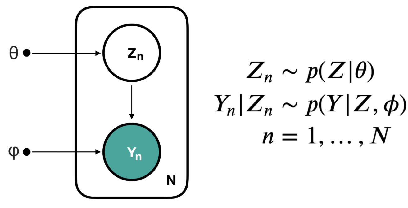
A graphic representation of the latent model, points are parameters, hollow circle is latent variable and solid circle is observed variable:
\(\begin{aligned}
Z_n &\sim P(Z | \theta) \\
Y_n &\sim P(Y| Z, \phi) \end{aligned}\tag{1}\)
The interpretation is that, a latentlatent means this variable is not observable, but it will determine the observables behaviour variable \(Z\) is subject to a distribution \(P(Z|\theta)\) parameterized by \(\theta\). For each data point \(n\), its observable variable \(Y_n\) is determined by the latent \(Z_n\) plus extra parameters \(\phi\): \(P(Y|Z,\phi)\).
Assume we have observed \(N\) data points \(\{y_n\}, n=1,\dots,N\). Our task is, given data \(\{y_n\}\), what are the most suitable parameters value \(\theta, \phi\) in the modelThis is a maximum likelihood point estimate task, we could also extend it to a probablistic target like \(p(\theta,\phi|y_n)\) or a posterior task \(p(Z_n|y_n)\), and add the prior information to make it bayesian ?
For example, a gaussian mixture model is a typical latent model: all data points are generated by a mixture of different gaussian distributions. We could only observe the coordinations of data points, which are \(Y_n\), but these variables are determined by the cluster this point belongs to, which is latent \(Z_n\) and unobservable. So a gaussian mixture model can be formalized as:
$$\begin{aligned}Z_n &\sim Cat(\pi)\\
Y_n|Z_n &\sim \mathcal{N}(\mu_{Z_n},\sigma^2_{Z_n})
\end{aligned}\tag{2}$$
where \(Cat\) is a catogorical distribution and \(\mathcal{N}\) is a guassian distribution.
The inference task is, given a bunch of observed data point positions, what are the best means and variances of all gaussian clusters? See sklearn's implementation to solve such task.
Generally, we want to maximize the observed likelihood of the model given data:
\[\begin{aligned}\log \prod_{n=1}^{N} P\left(y_{n} \mid \theta, \phi\right) &=\sum_{n=1}^{N} \log P\left(y_{n} \mid \theta, \phi\right) \\&=\sum_{n=1}^{N} \log \int p\left(y_{n} \mid z_{n}, \phi\right) p\left(z_{n} \mid \theta\right) d z_{n} \\&= \underbrace{\sum_{n=1}^{N} \log \underset{z_{n} \sim P\left(z_{n} \mid \theta\right)}{\mathbb{E}}\left[p\left(y_{n} \mid z_{n}, \phi\right)\right]}_{l_y(\theta,\phi)}\end{aligned}\tag{3}\]The \(l_y(\theta,\phi)\) is the observed likelihood, also called evidence. Our MLE target could be formalized as:
\[\begin{aligned} \phi_{M L E}, \theta_{M L E}&=\arg\max_{\theta, \phi} l_{y}(\theta, \phi) \\&= \arg\max _{\theta, \phi} \sum_{n=1}^{N} \log \underset{z_n\sim P\left(z_{n} \mid \theta\right)}{\mathbb{E}}\left[P\left(y_{n} \mid z_{n}, \phi\right)\right]\end{aligned}\tag{4}\]The computational trouble
As our inference target can be foramlized as a maximization task in equation (4), the practical solution to such issue involves gradient calculation, say we have to gradient \(l_y(\theta,\phi)\) with respect to \(\theta,\phi\):
\[\begin{aligned} \nabla_{\theta,\phi}l_{y}(\theta,\phi) &= \nabla_{\theta,\phi} \sum_{n=1}^{N} \log \underset{z_n\sim P\left(z_{n} \mid \theta\right)}{\mathbb{E}}\left[P\left(y_{n} \mid z_{n}, \phi\right)\right]\\ &= \sum_{n=1}^{N} \nabla_{\theta,\phi} \log \underset{z_n\sim P\left(z_{n} \mid \theta\right)}{\mathbb{E}}\left[P\left(y_{n} \mid z_{n}, \phi\right)\right] \\ &= \sum_{n=1}^{N} \frac{\nabla_{\theta,\phi} \underset{z_n\sim P\left(z_{n} \mid \theta\right)}{\mathbb{E}}\left[P\left(y_{n} \mid z_{n}, \phi\right)\right]}{\underset{z_n\sim P\left(z_{n} \mid \theta\right)}{\mathbb{E}}\left[P\left(y_{n} \mid z_{n}, \phi\right)\right]} \end{aligned}\tag{5}\]Look at the numerator of the last step The term \(\underset{z_n\sim P\left(z_{n} \mid \theta\right)}{\mathbb{E}}\left[P\left(y_{n} \mid z_{n}, \phi\right)\right]\) itself can be calcualted in a MC estimate approach , the gradient operator and the expectation operator are not commutable, as the \(\mathbb{E}\) has to do with the parameter \(\theta\). So the direct gradient of the evidence \(l_y(\theta,\phi)\) is almost computational impossible, we have to think another way out.
ELBO via an auxillary distribution
Here is how we construct ELBO, the main idea is to make the expectation operator irrelevant to the parameter \(\theta\) by introducing an auxillary distribution \(q(z)\): At the last step of deduction, we exchange \(\log\) and \(\mathbb{E}\), so \(q(Z)\) can not be cancelled out. Then the maximization has to be taken over \(q (Z)\) too.
\[\begin{aligned}\underset{\theta, \phi}{\mathrm{max}}\; l_y(\theta, \phi) &= \underset{\theta, \phi}{\mathrm{max}}\; \log \prod_{n=1}^N\int_{\Omega_Z} \left(\frac{p(y_n, z_n|\theta, \phi)}{q(z_n)}q(z_n)\right) dz\\&= \underset{\theta, \phi}{\mathrm{max}}\; \log\,\prod_{n=1}^N\mathbb{E}_{Z\sim q(Z)} \left[ \frac{p(y_n, Z|\theta, \phi)}{q(Z)}\right]\\&= \underset{\theta, \phi}{\mathrm{max}}\; \sum_{n=1}^N \log \mathbb{E}_{Z\sim q(Z)} \left[\,\left( \frac{p(y_n, Z|\theta, \phi)}{q(Z)}\right)\right]\\&\geq \underset{\theta, \phi, q}{\mathrm{max}}\; \underbrace{\sum_{n=1}^N\mathbb{E}_{Z_n\sim q(Z)} \left[ \log\,\left(\frac{p(y_n, Z_n|\theta, \phi)}{q(Z_n)}\right)\right]}_{ELBO(\theta, \phi, q)}, \quad (\text{Jensen's Inequality})\\\end{aligned}\tag{6}\]See, ELBO is the lower bound to our true evidence \(l_y(\theta,\phi)\), so when we change to maximize the ELBO, we are in some degree maximize the evidence. And as the expectation \(\mathbb{E}_{Z_n\sim q(Z)}\) in ELBO is no more related to \(\theta\), so we can gradient ELBO as the expectation operator and the gradient operator with respect to parameters are commutable:
\[\begin{aligned} \nabla_{\theta, \phi} ELBO(\theta, \phi, q) &= \nabla_{\theta, \phi} \sum_{n=1}^N\mathbb{E}_{Z_n\sim q(Z)} \left[ \log\,\left(\frac{p(y_n, Z_n|\theta, \phi)}{q(Z_n)}\right)\right] \\ &= \sum_{n=1}^N\mathbb{E}_{Z_n\sim q(Z)}\left[\nabla_{\theta, \phi} \log\,\left(\frac{p(y_n, Z_n|\theta, \phi)}{q(Z_n)}\right)\right] \end{aligned}\tag{7}\]We still have to maximize ELBO with respect to \(q(z)\), whose gradient is not commutable with the expectation operator. We will show how to solve this in the next section, an EM alogorithm.
Clearly, miaximizing the ELBO is not equal to maximizing the evidence. When ELBO is maximized, we can say the \(l_y(\theta,\phi)\) is as big, but can still be far from optimized, like the following picture:

Maximize ELBO – EM algorithm
As mentioned above, ELBO has to be maximized with respect to \(\theta,\phi\) and \(q\). As they are not correlatedThis is the same idea of mean field assumption in variational inference , we can optimize them in a coordinate ascent manner: optimize over degrees of freedom one by one. For a MLE task over a latent model, this is usually called EM (Expectation Maximization) algorithm: 
An illustration of the iterative EM algorithm to maximize ELBO
M-Step: Maximize \(\theta,\phi\), fix \(q^*\)
This is solved as discussed in equation (7)
$$\begin{aligned}\theta^*, \phi^* &= \underset{\theta, \phi}{\mathrm{max}}\; ELBO(\theta, \phi, q) = \underset{\theta, \phi}{\mathrm{max}}\; \sum_{n=1}^N\mathbb{E}_{Z_n\sim q(Z)} \left[ \log\,\left(\frac{p(y_n, Z_n|\theta, \phi)}{q(Z_n)}\right)\right]\\&= \underset{\theta, \phi}{\mathrm{max}}\; \sum_{n=1}^N \int_{\Omega_Z} \log\,\left(\frac{p(y_n, z_n|\theta, \phi)}{q(z_n)}\right)q(z_n) dz_n\\&= \underset{\theta, \phi}{\mathrm{max}}\; \sum_{n=1}^N \int_{\Omega_Z} \log\,\left(p(y_n, z_n|\theta, \phi)\right) q(z_n)dz_n - \underbrace{\int_{\Omega_Z} \log \left(q(z_n)\right)q(z_n) dz_n}_{\text{constant with respect to }\theta, \phi}\\&\equiv \underset{\theta, \phi}{\mathrm{max}}\;\sum_{n=1}^N \int_{\Omega_Z} \log\,\left(p(y_n, z_n|\theta, \phi)\right) q(z_n)dz_n\\&= \underset{\theta, \phi}{\mathrm{max}}\;\sum_{n=1}^N \mathbb{E}_{Z_n\sim q(Z)} \left[ \log\left(p(y_n, z_n|\theta, \phi)\right)\right]\end{aligned}$$
E-Step: Maximize \(q\), fix \(\theta^*,\phi^*\)
Rather than optimizing the ELBO with respect to q, which seems hard (as the gradient is not commutable with the expectation operator), we will argue that optimizing the ELBO is equivalent to optimizing another function of q, one whose optimum is easy for us to compute.
$$\begin{aligned}l_y(\theta, \phi) &- ELBO(\theta, \phi, q) \\&= \sum_{n=1}^N \log p(y_n| \theta, \phi) - \sum_{n=1}^N \int_{\Omega_Z} \log\left(\frac{p(y_n, z_n|\theta, \phi)}{q(z_n)}\right)q(z_n) dz_n\\&= \sum_{n=1}^N \int_{\Omega_Z} \log\left(p(y_n| \theta, \phi)\right) q(z_n) dz_n - \sum_{n=1}^N \int_{\Omega_Z} \log\left(\frac{p(y_n, z_n|\theta, \phi)}{q(z_n)}\right)q(z_n) dz_n\\&= \sum_{n=1}^N \int_{\Omega_Z} \left(\log\left(p(y_n| \theta, \phi)\right) - \log\left(\frac{p(y_n, z_n|\theta, \phi)}{q(z_n)}\right) \right)q(z_n) dz_n\\&= \sum_{n=1}^N \int_{\Omega_Z} \log\left(\frac{p(y_n| \theta, \phi)q(z_n)}{p(y_n, z_n|\theta, \phi)} \right)q(z_n) dz_n\\&= \sum_{n=1}^N \int_{\Omega_Z} \log\left(\frac{q(z_n)}{p(z_n| y_n, \theta, \phi)} \right)q(z_n) dz_n \\&= \sum_{n=1}^N D_{\text{KL}} \left[ q(z_n) \| p(z_n| y_n, \theta, \phi)\right].\end{aligned}$$
As \(l_y(\theta, \phi)\) is not a function of \(q\), so maximize the ELBO with respect to \(q\) is equivalent to minimize the KL divergence between \(q\) and posterior:
$$\underset{q}{\mathrm{argmax}}\, ELBO(\theta^*, \phi^*, q) = \underset{q}{\mathrm{argmin}}\sum_{n=1}^N D_{\text{KL}} \left[ q(z_n) \| p(z_n| y_n, \theta^*, \phi^*)\right].$$
So we could just choose \(q^*\) to be the posteriorSometimes the posterior is intractable as it involves an integration over the whole latent space, e.g. VAE. We have to use variational inference tools to approximate the posterior. :
$$\begin{aligned}q^*(z_n) &= \underset{q}{\mathrm{argmax}}\; ELBO(\theta^*, \phi^*, q) \\&= \underset{q}{\mathrm{argmin}}\sum_{n=1}^N D_{\text{KL}} \left[ q(z_n) \| p(z_n| y_n, \theta^*, \phi^*)\right] \\&= p(z_n| y_n, \theta^*, \phi^*)\end{aligned}$$
- Initialization: pick \(\theta_0\), \(\phi_0\)
- Repeat \(i = 1,\dots,I\) times:
E-step:
\(q_{\text{new}}(Z_n) = \underset{q}{\mathrm{argmax}}\; ELBO(\theta_{\text{old}}, \phi_{\text{old}}, q) = p(Z_n|Y_n, \theta_{\text{old}}, \phi_{\text{old}})\)
M-step:
\(\begin{aligned} \theta_{\text{new}}, \phi_{\text{new}} &= \underset{\theta, \phi}{\mathrm{argmax}}\; ELBO(\theta, \phi, q_{\text{new}})\\ &= \underset{\theta, \phi}{\mathrm{argmax}}\; \sum_{n=1}^N\mathbb{E}_{Z_n\sim p(Z_n|Y_n, \theta_{\text{old}}, \phi_{\text{old}})}\left[\log \left( p(y_n, Z_n | \phi, \theta\right) \right]. \end{aligned}\)