ODE and PDE, Nonhomogeneous ODEs
February 18, 2021
1. Methods of undetermined coefficients
For a nonhomogeneous second-order ODE:
\[y^{\prime \prime}+p(t) y^{\prime}+q(t) y=g(t) \tag{1}\]where \(g(t)\) is nonzero. We can write out the general solution as:
\[y=\phi(t)=c_{1} y_{1}(t)+c_{2} y_{2}(t)+Y(t)\tag{2}\]\(y_1\) and \(y_2\) are the two solutions for the homogeneous formset \(g(t)=0\) of equation (1). Our task now is finding the specific solution \(Y(t)\).
Say, if \(g(t)\) involves only polynomials, sines, cosines, or exponential functions, or sums or products of any of these functions.Think about why. Take equation (2) back to (1)
We can get the general solution with the following four steps:
-
Get the solution to the homogeneous equation \(y_1(t)\) and \(y_2(t)\)
-
Assume an appropriate form for the particular solution \(Y(t) .\) If \(g(t)=\exp (\alpha t),\) assume \(Y(t)=\) \(A \exp (\alpha t) .\) If \(g(t)=\sin (\beta t)\) or \(\cos (\beta t),\) assume \(Y(t)=A \cos (\beta t)+B \sin (\beta t) .\) If \(g(t)\) is a polynomial of order \(n,\) then assume \(Y(t)\) is a polynomial of order \(n\). If \(g(t)\) is a sum or product of the aforementioned functions, assume \(Y(t)\) is also a sum or product of those same functions. It may be necessary to multiply by \(t\) or \(t^{2}\) to avoid duplicating the homogeneous solution.
-
Plug the assumed \(Y (t)\) into the differential equation to determine the necessary coefficients.
-
Take the sum of the homogeneous and particular solutions to get the general solution of the non-homogeneous differential equation.
2. Variation of parameters
If \(g(t)\) is not the case mentioned above, we need a more general method to solve, here are the general solution for equation (1):
\[y=c_{1} y_{1}(t)+c_{2} y_{2}(t)+u_{1}(t) y_{1}(t)+u_{2}(t) y_{2}(t)\tag{3}\]\(y_1\) and \(y_2\) are the two solutions for the homogeneous formset \(g(t)=0\) of equation (1).
where:
\[u_{1}(t)=-\int \frac{y_{2}(t) g(t)}{W\left[y_{1}, y_{2}\right](t)} d t , \ u_{2}(t)=\int \frac{y_{1}(t) g(t)}{W\left[y_{1}, y_{2}\right](t)} d t \tag{4}\]and the Wronskian is:
\[W\left[y_{1}, y_{2}\right](t)=\left|\begin{array}{ll} y_{1}(t) & y_{2}(t) \\ y_{1}^{\prime}(t) & y_{2}^{\prime}(t) \end{array}\right|=y_{1}(t) y_{2}^{\prime}(t)-y_{1}^{\prime}(t) y_{2}(t)\tag{5}\]3. Forced Vibration
The typical example of 2nd Nonhomogeneous ODE is forced periodic vibrations. Assume a general spring-mass system is subject to an external force \(F(t)\)\(\gamma\) is damping force, k is spring constant, m is mass :
\[m u^{\prime \prime}(t)+\gamma u^{\prime}(t)+k u(t)=F(t)=F_{0} \cos (\omega t)\tag{6}\]The general solution must have the form:
\[u=c_{1} u_{1}(t)+c_{2} u_{2}(t)+A \cos (\omega t)+B \sin (\omega t)=u_{c}(t)+U(t) \tag{7}\]The solution \(u_1(t)\) and \(u_{2}(t)\) of the homogeneous equation depend on the roots \(r_{1}\) and \(r_{2}\) of the characteristic equation \(m r^{2}+\gamma r+k=0 .\) Since \(m, \gamma\), and \(k\) are all positive, it follows that \(r_{1}\) and \(r_{2}\) either are real and negative or are complex conjugates with a negative real partThink about why . In either case, both \(u_{1}(t)\) and \(u_{2}(t)\) approach zero as \(t \rightarrow \infty\). Since \(u_{c}(t)\) dies out as \(t\) increases, it is called the transient solutionIn many applications, it is of little importance and (depending on the value of \(\gamma\) ) may well be undetectable after only a few seconds. .
\(U(t)\) represents a steady oscillation with the same frequency as the external force and are called the steady-state solution or the forced response of the system, which can be written as:
\[U(t)=R \cos (\omega t-\delta)\tag{8}\]The amplitude \(R\) and phase \(\delta\) are:
\[R=\frac{F_{0}}{\Delta}, \quad \cos \delta=\frac{m\left(\omega_{0}^{2}-\omega^{2}\right)}{\Delta}, \quad \text{and} \quad \sin \delta=\frac{\gamma \omega}{\Delta} \tag{9}\]where
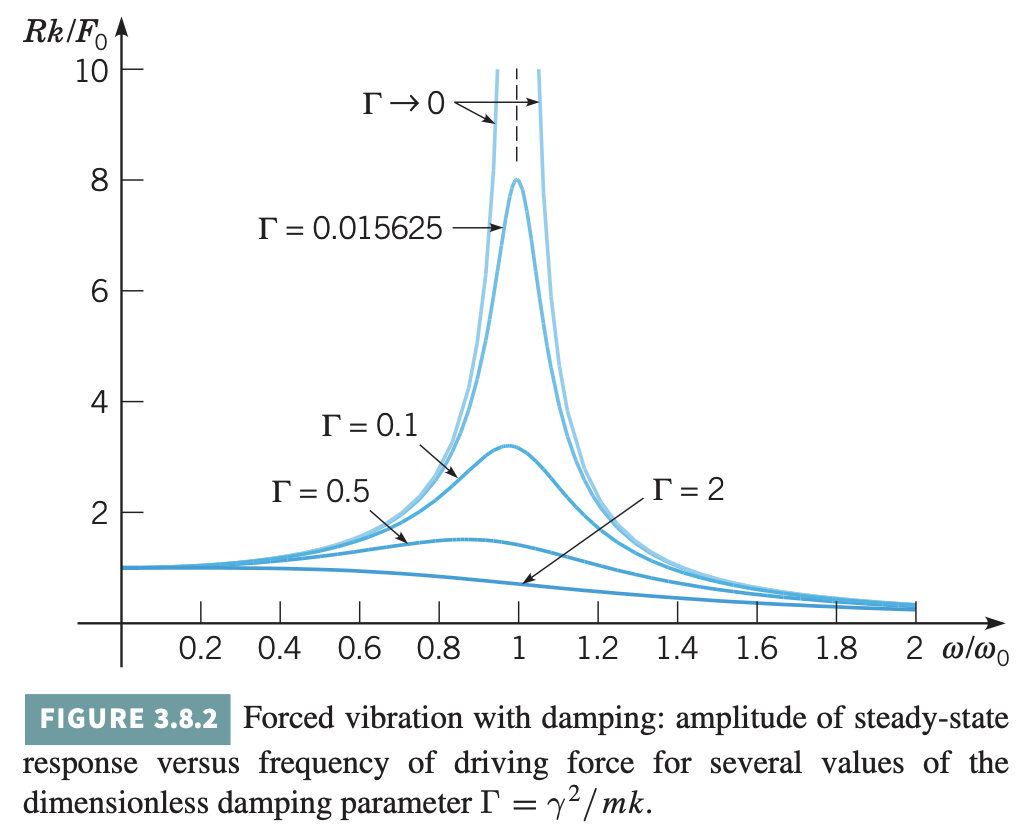
\[\Delta=\sqrt{m^{2}\left(\omega_{0}^{2}-\omega^{2}\right)^{2}+\gamma^{2} \omega^{2}} \quad \text{and} \quad \omega_{0}^{2}=\frac{k}{m}\tag{10}\]We now investigate how the amplitude \(R\) of the steady-state oscillation depends on the frequency \(\omega\) of the external force. With some alegebra, we find that:
\[\frac{R k}{F_{0}}=\left(\left(1-\left(\frac{\omega}{\omega_{0}}\right)^{2}\right)^{2}+\Gamma\left(\frac{\omega}{\omega_{0}}\right)^{2}\right)^{-1 / 2} \text { where } \Gamma=\frac{\gamma^{2}}{m k}\]For low frequency excitation -$that is, as \(\omega \rightarrow 0\) -it follows that \(R k / F_{0} \rightarrow 1\) or \(R \rightarrow F_{0} / k .\) At the other extreme, for very high frequency excitation, \(R \rightarrow 0\) as \(\omega \rightarrow \infty\). At an intermediate value of \(\omega = \omega_{\max}\) the amplitude may have a maximum:
\[\omega_{\max }^{2}=\omega_{0}^{2}-\frac{\gamma^{2}}{2 m^{2}}=\omega_{0}^{2}\left(1-\frac{\gamma^{2}}{2 m k}\right)\]Note that \(\omega_{\max }<\omega_{0}\) and that \(\omega_{\max }\) is close to \(\omega_{0}\) when \(\gamma\) is small. The maximum value of \(R\) is:
\[R_{\max }=\frac{F_{0}}{\gamma \omega_{0} \sqrt{1-\left(\gamma^{2} / 4 m k\right)}} \cong \frac{F_{0}}{\gamma \omega_{0}}\left(1+\frac{\gamma^{2}}{8 m k}\right)\]where the last expression is an approximation that is valid when \(\gamma\) is small. If \(\frac{\gamma^{2}}{m k}>2\), then \(\omega_{\max }\) is imaginary; in this case the maximum value of \(R\) occurs for \(\omega=0\), and \(R\) is a monotone decreasing function of \(\omega .\) Recall that critical damping occurs when \(\frac{\gamma^{2}}{m k}=4\).