ODE and PDE, Basics I
January 15, 2021
- 1. Classification of Differential Equations
- 2. Order and Solutions
- 3. First-Order Linear ODE: Integrating Factors
- 4. Initial value problem (IVP)
1. Classification of Differential Equations
Only ordinary derivatives appear in the differential equation, and it is said to be an ordinary differential equation (ODE), like:
\[L \frac{d^{2} Q(t)}{d t^{2}}+R \frac{d Q(t)}{d t}+\frac{1}{C} Q(t)=E(t) \tag{1.1}\]the derivatives are partial derivatives, and the equation is called a partial differential equation(PDE), like:
\[\alpha^{2} \frac{\partial^{2} u(x, t)}{\partial x^{2}}=\frac{\partial u(x, t)}{\partial t} \tag{1.2}\]Let’s focus on ODE at this moment. For an ODE:
\[F\left(t, y, y^{\prime}, \ldots, y^{(n)}\right)=0 \tag{1.3}\]where \(F\) is a linear function of the variables \(y, y', \dots, y^{(n)}\), like:
\[F(\cdot)= a_{0}(t) y^{(n)}+a_{1}(t) y^{(n-1)}+\cdots+a_{n}(t) y+g(t) = 0\tag{1.4}\]This ODE is said to be linear. An equation which is not in the form of equation (1.4) is nonlinear, like an oscillating pendulum system in physics:
\[\frac{d^{2} \theta}{d t^{2}}+\frac{g}{L} \sin \theta=0 \tag{1.5}\]The \(\sin\theta\) term is nonlinear.
2. Order and Solutions
The order of a differential equation is the order of the highest derivative that appears in the equation. Generally speaking,
\[F\left(t, u(t), u^{\prime}(t), \ldots, u^{(n)}(t)\right)=0 \tag{2.1}\]is a \(n^{th}\) order ODE.
A solution of the \(n^{th}\) order ODE on the interval \(\alpha< t < \beta\) is a function \(\phi\) such that \(\phi', \phi'',\dots, \phi^{(n)}\) exist and satisfy:
\[\phi^{(n)}(t)=f\left(t, \phi(t), \phi^{\prime}(t), \ldots, \phi^{(n-1)}(t)\right)\tag{2.2}\]for every \(t\) in \(\alpha< t < \beta\).
Existence and uniqueness are two important questions of differential equation solutions that we are interested in. Existence is the qeustion to answer if the equation has a solution, and uniqueness is trying to answer how many solutions it has. In general, solutions of differential equations contain one or more arbitrary constants of integration. So a following third question, which is also important, is how can we actually determine a solution of a differential equation? We need the help of initial value or boundary conditions.
3. First-Order Linear ODE: Integrating Factors
Let’s dive into a discussion about how to solve first-order linear ODE. In general, a first-order linear ODE can be written in the form:
\[P(t) \frac{d y}{d t}+Q(t) y=G(t)\tag{3.1}\]where \(P\), \(Q\), and \(G\) are given as functions of independent variable \(t\). Trivially, as long as \(P(t)\ne 0\)or it is not a first-order ODE , the equation (3.1) can be converted into the following form by dividing both sides by \(P(t)\):
\[\frac{d y}{d t}+p(t) y=g(t)\tag{3.2}\]In some case, a first-order linear ODE can be solved easily by integrating the equation, likeBoyce book, Page 25, Section 2.1, Example 1 : $$ \left(4+t^{2}\right) \frac{d y}{d t}+2 t y=4 t\tag{3.3} $$ can be solved immediately: $$ (3.3)\implies\frac{d}{d t}\left(\left(4+t^{2}\right) y\right)=4 t\implies\left(4+t^{2}\right) y=2 t^{2}+c\\ \implies y=\frac{2 t^{2}}{4+t^{2}}+\frac{c}{4+t^{2}} $$
The above solution method requires the linear ODEs have the property that their left-hand sides can be written as the derivative of the product of y and some other function, meaning a ODE in form (3.1) satisfies:
\[\frac{d}{dt}[P(t)y]=P(t)\frac{dy}{dt}+Q(t)y \implies \frac{dP(t)}{dt}=Q(t)\tag{3.4}\]Unfortunately, most first-order linear differential equations do not have such property. However, as discovered by Leibniz, we can multiply the differential equation by a certain function \(\mu(t)\):
\[P(t) \frac{d y}{d t}+Q(t) y=G(t)\\ \implies P(t)\mu(t) \frac{d y}{d t}+Q(t)\mu(t) y=G(t)\mu(t) \tag{3.5}\]then the new linear ODE could satisify the property (3.4), such that:
\[\frac{d}{dt}[P(t)\mu(t)]=Q(t)\mu(t)\tag{3.6}\]Then the new ODE (3.5) can be solved with the immediate integrating method. The function \(\mu(t)\) is called integrating factors and our task now shifts to finding a function \(\mu(t)\) to make equation (3.6) true.
Rewrite the equation (3.6) with the product rule for derivativesThink about the conditions to make the following deductions true. :
\[P(t)\frac{d}{dt}\mu(t) + \mu(t)\frac{d}{dt}P(t) = Q(t)\mu(t)\\[2ex] \implies [Q(t)-\frac{d}{dt}P(t)]\mu(t) = P(t)\frac{d}{dt}\mu(t)\\[2ex] \implies \frac{Q(t)}{P(t)} - \frac{1}{P(t)}\frac{dP(t)}{dt} = \frac{1}{\mu(t)}\frac{d\mu(t)}{dt}\\[2ex] \implies \frac{Q(t)}{P(t)}dt - \frac{dP(t)}{P(t)} = \frac{d\mu(t)}{\mu(t)}\\ \implies \int \frac{Q(t)}{P(t)} dt - \ln P(t) + \text{Const} = \ln \mu(t) \tag{3.7}\]So we have the integrating factor form:
\[\mu(t) = Ce^{\int \frac{Q(t)}{P(t)} dt - \ln P(t)}\tag{3.8}\]where C is a constant. If we use the ODE form (3.2), or where \(P(t) = 1\) and \(Q(t)=p(t)\), then the integrating factor isThis is the same as Boyce book Page 28, Equation 30 :
\[\mu(t) = Ce^{\int p(t)dt}\tag{3.9}\]Multiply both side of Equation (3.2) by (3.9) then integrate, we can find a general solution to equation (3.3)Think about if and when could this general solution fail? :
\[y=\frac{1}{\mu(t)}\left(\int_{t_{0}}^{t} \mu(s) g(s) d s+c\right)\tag{3.10}\]where we have to intergrate out \(\mu(t)\) by equation (3.9) You can drop the constant C in equation (3.9) at the moment , then use (3.10). The lower limit \(t_0\) as well as the constant \(c\) is determined by given initial value.
4. Initial value problem (IVP)
As you might have mentioned above, direct solving of differential equations always involves some undertermined constants. The ituition for this phenomenon is, a differention operation applied to any constant would always give 0, so you can’t tell the difference about two constants from a differentiated equations. This is usually solved by the given initial value.
Think about the example 5 on Boyce book page 30, we want to solve the equation:
\[2y'+ty=2\tag{4.1}\]With the intergrating factor tool we established last section, the solution is:
\[y=e^{-t^{2} / 4} \int_{0}^{t} e^{s^{2} / 4} d s+c e^{-t^{2} / 4}\tag{4.2}\]See, an undetermined constant \(c\) here. So here we need another fact, which is called Initial Valueor boundary condition in higher dimensional, or more physics-related, problems , like:
\[y(0)=1 \tag{4.3}\]Take this into (4.2), we could simply solve \(c=1\). This can be illustrated with the figure
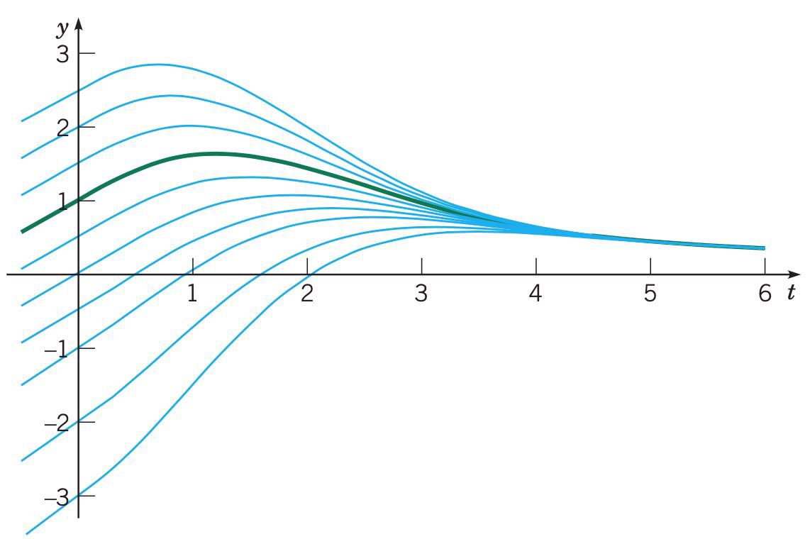
As all the curves satisfy the solution (4.2), but only the green one meets the initial value \(y(0)=1\).