And the maximum likelihood training tagets writes:
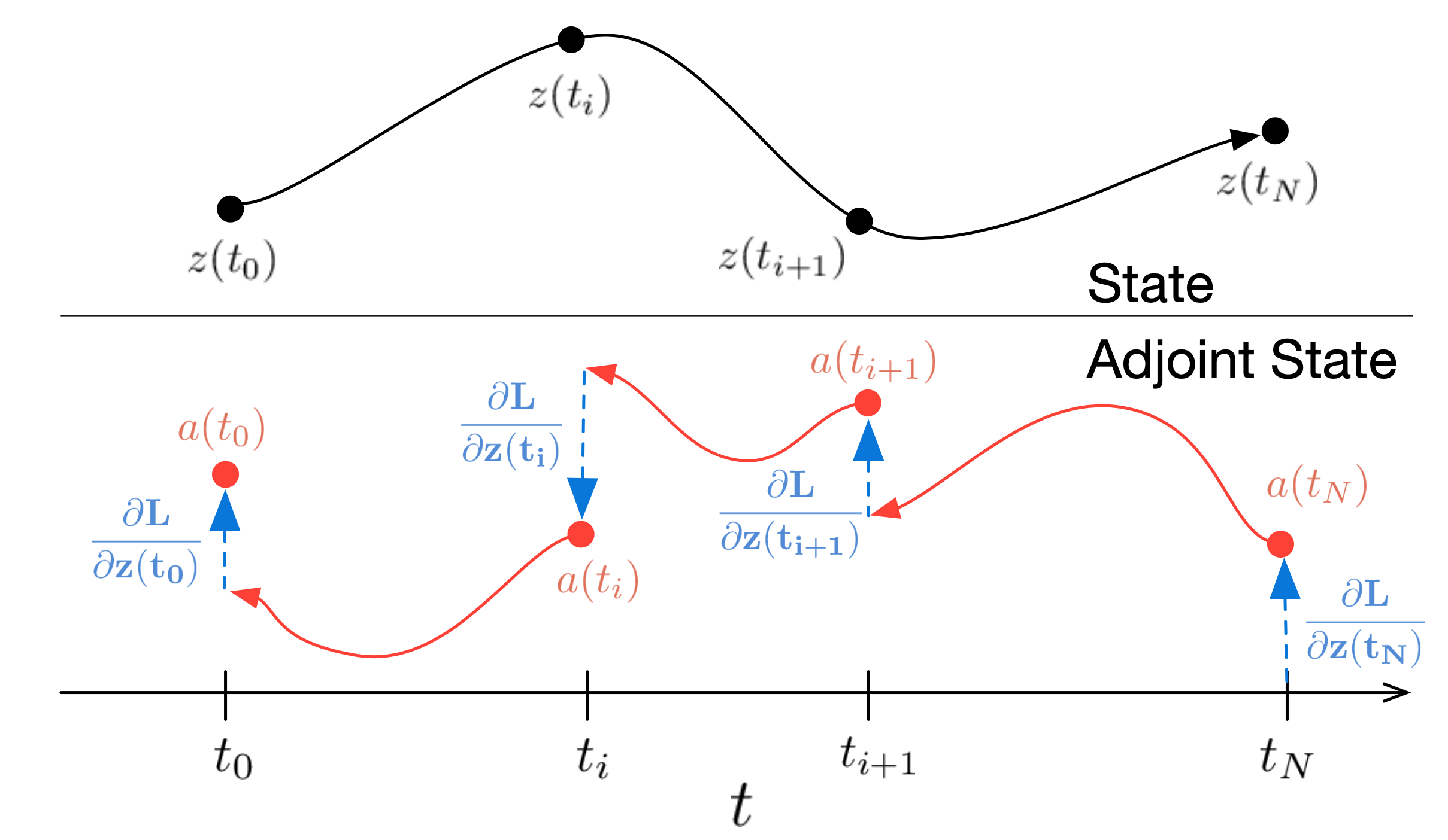
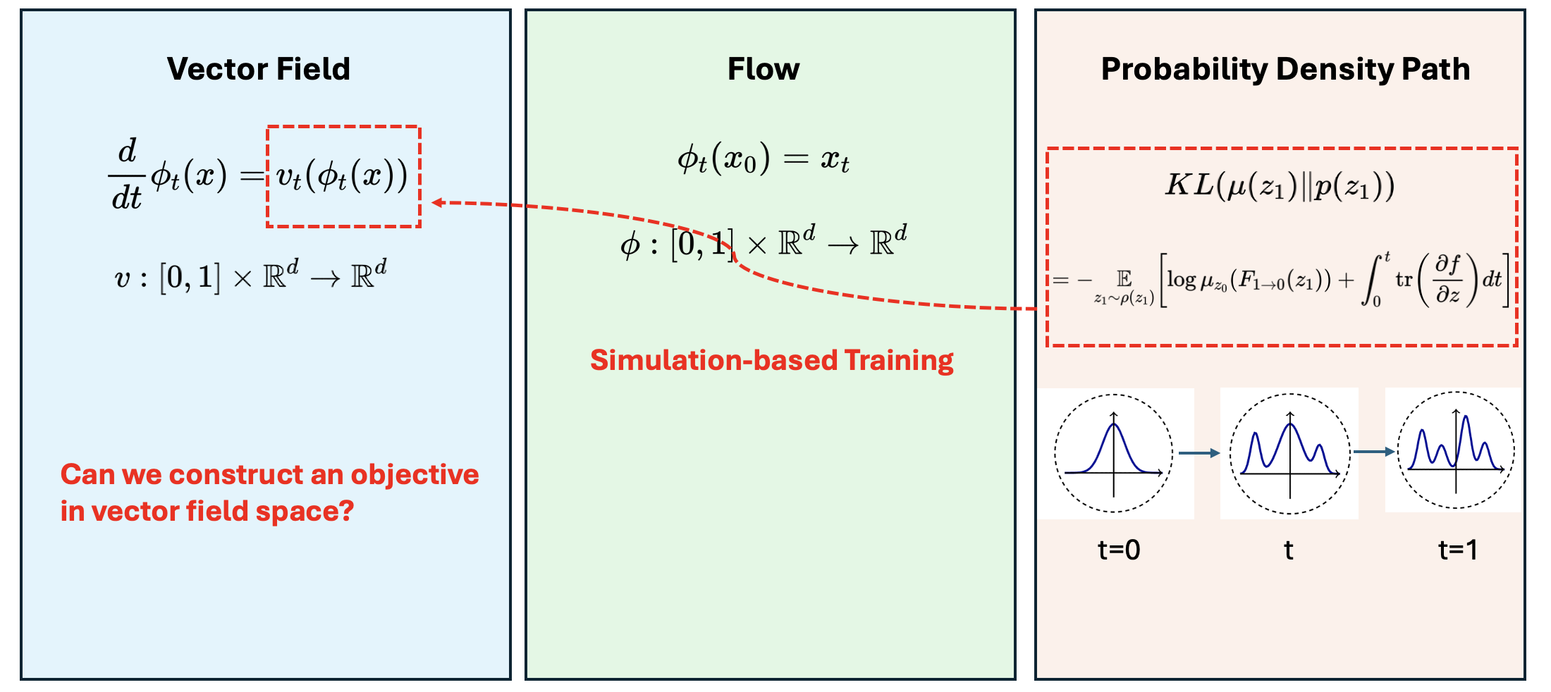
\[-\underset{z_1 \sim \rho\left(z_1\right)}{\mathbb{E}}\left[\log \mu_{z_0}\left(F_{1 \rightarrow 0}\left(z_1\right)\right)+\int_0^1 \operatorname{tr}\left(\frac{\partial f}{\partial z}\right) d t\right]\]The adjoint method training would require several ODEsolver runs for each iteration, which is not scalable. How to make an affordable training protocol?
Vector field, flow and probability density path
Before we move on to the flow-matching objective, let’s first clarify three concepts: vector field, flow and probability density path. They can be understood as three different representations of variable transformation.
Say we have variable \(x_0 \in \mathbb{R}^d\), with probability distibution \(p_0\)
-
Flow \(\phi\)
Flow is the transformation of the variable into another variable with the same dimensionality:
\[\begin{gathered} \phi_t\left(x_0\right)=x_t \\ \phi:[0,1] \times \mathbb{R}^d \rightarrow \mathbb{R}^d \end{gathered} \tag{1}\] -
Probability Density Path \(p_t\)
Under the above flow transformation, the probability density function of the transformed variable would change as well:
\[\begin{gathered} p_t=\left[\phi_t\right]_* p_0 \\ p:[0,1] \times \mathbb{R}^d \rightarrow \mathbb{R}_{>0} \end{gathered}\tag{2}\]With the change of variables theorem, we know the density function changes as following:
\[\left[\phi_t\right]_* p_0(x)=p_0\left(\phi_t^{-1}(x)\right) \operatorname{det}\left[\frac{\partial \phi_t^{-1}}{\partial x}(x)\right]\tag{3}\] -
Vector Field \(v_t\)
If we say the above flow/transformation is constructed by a neural ODE, then it could be written as:
\[\begin{aligned} & \frac{d}{d t} \phi_t(x)=v_t\left(\phi_t(x); \theta\right) \\ & v:[0,1] \times \mathbb{R}^d \rightarrow \mathbb{R}^d \end{aligned}\tag{4}\]\(v\) is parameterized by neural network \(\theta\).
In the simulation-based training protocol for continuous normalizing flow, our target lives in the probability density path representation, but our parameters are in the vector field space. Connecting that two representations are expensive. Can we directly construct an objective in vector field space, so the training can be more in a regression manner?
Flow Matching Objective
Say we have samples from unknown distribution \(q(x_1)\). We hope to have a probability density path \(p_t(x)\), such that we can transform a simple distribution to approximate the underlying complex distribution:
\[p_0(x)=p(x)=\mathcal{N}(x \mid 0, I) \qquad \text{at t=0}\tag{5}\] \[p_1(x) \approx q(x) \qquad \text{at t=1} \tag{6}\]And such path could be constructed by a corresponding vector field \(u_t(x)\), so idealy we could use the following Flow Matching Objective: to train our vector field:
\[\mathcal{L}_{\mathrm{FM}}(\theta)=\mathbb{E}_{t, p_t(x)}\left\|v_t(x, \theta)-u_t(x)\right\|^2\tag{7}\]Unfortunately we don’t know how to sample from \(p_t(x)\), neither do we know the exact form of ground truth \(u_t(x)\).
Conditional Flow Matching
To tackle the above issue, now we define a conditioanl probability path \(p_t\left(x \mid x_1\right)\), such that it could trasform a simple distribution function into a narrow gaussian around \(x_1\):
\[p_0\left(x \mid x_1\right)=p(x)=\mathcal{N}(x \mid 0, I) \qquad \text{at t=0}\tag{8}\] \[p_1\left(x \mid x_1\right)=\mathcal{N}\left(x \mid x_1, \sigma^2 I\right) \qquad \text{at t=1} \tag{9}\]The corresponding marginal path is:
\[p_t(x)=\int p_t\left(x \mid x_1\right) q\left(x_1\right) d x_1\tag{10}\]And as \(\sigma \to 0\), we can easily prove:
\[p_1(x)=\int p_1\left(x \mid x_1\right) q\left(x_1\right) d x_1 \approx q(x)\]Let’s say conditonal proability path could be constructed by a conditonal vector field \(u_t\left(x \mid x_1\right)\), and it would aggregate to be the marginal vector field:
\[u_t(x)=\int u_t\left(x \mid x_1\right) \frac{p_t\left(x \mid x_1\right) q\left(x_1\right)}{p_t(x)} d x_1 \tag{11}\]In the theorem 1 of the original paper, they proved that the marginal vector field could construct marginal density path.
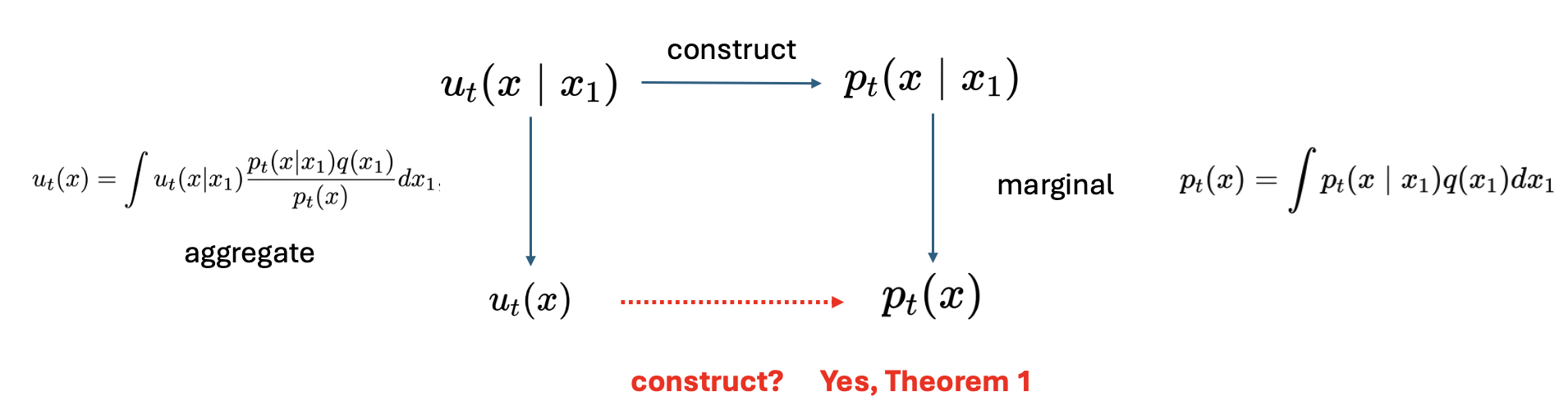
However, even though we have the equation (10) and (11) for \(p_t(x)\) and \(u_t(x)\), the \(\mathcal{L}_{\mathrm{FM}}(\theta)\) in equation (7) is still intractable because of the integrals in (10) and (11).
Conditional Flow Matching Objective
Instead we can define the following conditional flow matching objective:
\[\mathcal{L}_{\mathrm{CFM}}(\theta)=\mathbb{E}_{t, q\left(x_1\right), \textcolor{#e41a1c}{p_t\left(x \mid x_1\right)}}\left\|v_t(x, \theta)-\textcolor{#377eb8}{u_t\left(x \mid x_1\right)}\right\|^2 \tag{12}\]And in their theorem 2, the authors proved that:
\[\nabla_\theta \mathcal{L}_{F M}(\theta)=\nabla_\theta \mathcal{L}_{C F M}(\theta) \tag{13}\]So minimizing CFM with gradient descent is the same as miminizing FM target. And the conditional path and vector filed in the CFM do not involve any integrals, we only have to determine the form of \(p_t\left(x \mid x_1\right)\) and \(u_t\left(x \mid x_1\right)\) based on our choice.
We consider a gaussian conditional probability path:
\[\textcolor{#e41a1c}{p_t\left(x \mid x_1\right)=\mathcal{N}\left(x \mid \mu_t\left(x_1\right), \sigma_t\left(x_1\right)^2 I\right)} \tag{14}\]with
\[\mu_0\left(x_1\right)=0, \sigma_0\left(x_1\right)=1 \qquad \text{at t = 0}\] \[\mu_0\left(x_1\right)=x_1, \sigma_0\left(x_1\right)=\sigma_{\text{min}} \qquad \text{at t = 0}\]And the corresponding flow is \(\psi_t(x)=\sigma_t\left(x_1\right) x+\mu_t\left(x_1\right)\)
According to the theorem 3, we have the expression of the confitional vector field:
\[\textcolor{#377eb8}{u_t\left(x \mid x_1\right)=\frac{\sigma_t^{\prime}\left(x_1\right)}{\sigma_t\left(x_1\right)}\left(x-\mu_t\left(x_1\right)\right)+\mu_t^{\prime}\left(x_1\right)} \tag{15}\]Then the only missing pieces for calculating CFM in (12) are \(\mu_t\left(x_1\right)\) and \(\sigma_t\left(x_1\right)\) in equation (14). They depends on our choices of different paths.
Consider two different diffusion paths
1. Data to noise
$$
\mu_t\left(x_1\right)=x_1 \quad \sigma_t\left(x_1\right)=\sigma_{1-t}
$$
$$
u_t\left(x \mid x_1\right)=-\frac{\sigma_{1-t}^{\prime}}{\sigma_{1-t}}\left(x-x_1\right)
$$
2. Noise to data
$$
\mu_t\left(x_1\right)=\alpha_{1-t} x_1 \quad \sigma_t\left(x_1\right)=\sqrt{1-\alpha_{1-t}^2}
$$
$$
u_t\left(x \mid x_1\right)=\frac{\alpha_{1-t}^{\prime}}{1-\alpha_{1-t}^2}\left(\alpha_{1-t} x-x_1\right)=-\frac{T^{\prime}(1-t)}{2}\left[\frac{e^{-T(1-t)} x-e^{-\frac{1}{2} T(1-t)} x_1}{1-e^{-T(1-t)}}\right]
$$
Consider the optimal transportation path
$$
\mu_t(x)=t x_1 \text {, and } \sigma_t(x)=1-\left(1-\sigma_{\min }\right) t
$$
$$
u_t\left(x \mid x_1\right)=\frac{x_1-\left(1-\sigma_{\min }\right) x}{1-\left(1-\sigma_{\min }\right) t}
$$
$$
\mathcal{L}_{\mathrm{CFM}}(\theta)=\mathbb{E}_{t, q\left(x_1\right), p\left(x_0\right)}\left\|v_t\left(\psi_t\left(x_0\right)\right)-\left(x_1-\left(1-\sigma_{\text {min }}\right) x_0\right)\right\|^2
$$